Introduction
As the name suggests, random forest models basically contain an ensemble of decision tree models, with each decision tree predicting the same response variable. The response may be categorical, in which case being a classification problem, or continuous / numerical, being a regression problem.
In this short tutorial, we will go through the use of tree-based methods (decision tree, bagging model, and random forest) for both classification and regression problems.
This tutorial is divided into two sections. We will first use tree-based methods for classification on the spam dataset from the kernlab package. Subsequently, we will apply these methods on a regression problem, with the imports85 dataset from the randomForest package.
Tree-based methods for classification
Preparation
Let’s start by loading the spam dataset and doing some preparations:
# packages that we will need:
#  @ kernlab:      for the spam dataset
#  @ tree:         for decision tree construction
#  @ randomForest: for bagging and RF
#  @ beepr:        for a little beep
#  @ pROC:         for plotting of ROC

# code snippet to install and load multiple packages at once
# pkgs <- c("kernlab","tree","randomForest","beepr","pROC")
# sapply(pkgs,FUN=function(p){
#        print(p)
#        if(!require(p)) install.packages(p)
#        require(p)
# })

# load required packages
suppressWarnings(library(kernlab))
suppressWarnings(library(tree))
suppressWarnings(library(randomForest))
## randomForest 4.6-14
## Type rfNews() to see new features/changes/bug fixes.
suppressWarnings(library(beepr)) # try it! beep()
suppressWarnings(library(pROC))
## Type 'citation("pROC")' for a citation.
##
## Attaching package: 'pROC'
## The following objects are masked from 'package:stats':
##
##     cov, smooth, var

# load dataset
data(spam)

# take a look
str(spam)
## 'data.frame':    4601 obs. of  58 variables:
##  $ make             : num  0 0.21 0.06 0 0 0 0 0 0.15 0.06 ...
##  $ address          : num  0.64 0.28 0 0 0 0 0 0 0 0.12 ...
##  $ all              : num  0.64 0.5 0.71 0 0 0 0 0 0.46 0.77 ...
##  $ num3d            : num  0 0 0 0 0 0 0 0 0 0 ...
##  $ our              : num  0.32 0.14 1.23 0.63 0.63 1.85 1.92 1.88 0.61 0.19 ...
##  $ over             : num  0 0.28 0.19 0 0 0 0 0 0 0.32 ...
##  $ remove           : num  0 0.21 0.19 0.31 0.31 0 0 0 0.3 0.38 ...
##  $ internet         : num  0 0.07 0.12 0.63 0.63 1.85 0 1.88 0 0 ...
##  $ order            : num  0 0 0.64 0.31 0.31 0 0 0 0.92 0.06 ...
##  $ mail             : num  0 0.94 0.25 0.63 0.63 0 0.64 0 0.76 0 ...
##  $ receive          : num  0 0.21 0.38 0.31 0.31 0 0.96 0 0.76 0 ...
##  $ will             : num  0.64 0.79 0.45 0.31 0.31 0 1.28 0 0.92 0.64 ...
##  $ people           : num  0 0.65 0.12 0.31 0.31 0 0 0 0 0.25 ...
##  $ report           : num  0 0.21 0 0 0 0 0 0 0 0 ...
##  $ addresses        : num  0 0.14 1.75 0 0 0 0 0 0 0.12 ...
##  $ free             : num  0.32 0.14 0.06 0.31 0.31 0 0.96 0 0 0 ...
##  $ business         : num  0 0.07 0.06 0 0 0 0 0 0 0 ...
##  $ email            : num  1.29 0.28 1.03 0 0 0 0.32 0 0.15 0.12 ...
##  $ you              : num  1.93 3.47 1.36 3.18 3.18 0 3.85 0 1.23 1.67 ...
##  $ credit           : num  0 0 0.32 0 0 0 0 0 3.53 0.06 ...
##  $ your             : num  0.96 1.59 0.51 0.31 0.31 0 0.64 0 2 0.71 ...
##  $ font             : num  0 0 0 0 0 0 0 0 0 0 ...
##  $ num000           : num  0 0.43 1.16 0 0 0 0 0 0 0.19 ...
##  $ money            : num  0 0.43 0.06 0 0 0 0 0 0.15 0 ...
##  $ hp               : num  0 0 0 0 0 0 0 0 0 0 ...
##  $ hpl              : num  0 0 0 0 0 0 0 0 0 0 ...
##  $ george           : num  0 0 0 0 0 0 0 0 0 0 ...
##  $ num650           : num  0 0 0 0 0 0 0 0 0 0 ...
##  $ lab              : num  0 0 0 0 0 0 0 0 0 0 ...
##  $ labs             : num  0 0 0 0 0 0 0 0 0 0 ...
##  $ telnet           : num  0 0 0 0 0 0 0 0 0 0 ...
##  $ num857           : num  0 0 0 0 0 0 0 0 0 0 ...
##  $ data             : num  0 0 0 0 0 0 0 0 0.15 0 ...
##  $ num415           : num  0 0 0 0 0 0 0 0 0 0 ...
##  $ num85            : num  0 0 0 0 0 0 0 0 0 0 ...
##  $ technology       : num  0 0 0 0 0 0 0 0 0 0 ...
##  $ num1999          : num  0 0.07 0 0 0 0 0 0 0 0 ...
##  $ parts            : num  0 0 0 0 0 0 0 0 0 0 ...
##  $ pm               : num  0 0 0 0 0 0 0 0 0 0 ...
##  $ direct           : num  0 0 0.06 0 0 0 0 0 0 0 ...
##  $ cs               : num  0 0 0 0 0 0 0 0 0 0 ...
##  $ meeting          : num  0 0 0 0 0 0 0 0 0 0 ...
##  $ original         : num  0 0 0.12 0 0 0 0 0 0.3 0 ...
##  $ project          : num  0 0 0 0 0 0 0 0 0 0.06 ...
##  $ re               : num  0 0 0.06 0 0 0 0 0 0 0 ...
##  $ edu              : num  0 0 0.06 0 0 0 0 0 0 0 ...
##  $ table            : num  0 0 0 0 0 0 0 0 0 0 ...
##  $ conference       : num  0 0 0 0 0 0 0 0 0 0 ...
##  $ charSemicolon    : num  0 0 0.01 0 0 0 0 0 0 0.04 ...
##  $ charRoundbracket : num  0 0.132 0.143 0.137 0.135 0.223 0.054 0.206 0.271 0.03 ...
##  $ charSquarebracket: num  0 0 0 0 0 0 0 0 0 0 ...
##  $ charExclamation  : num  0.778 0.372 0.276 0.137 0.135 0 0.164 0 0.181 0.244 ...
##  $ charDollar       : num  0 0.18 0.184 0 0 0 0.054 0 0.203 0.081 ...
##  $ charHash         : num  0 0.048 0.01 0 0 0 0 0 0.022 0 ...
##  $ capitalAve       : num  3.76 5.11 9.82 3.54 3.54 ...
##  $ capitalLong      : num  61 101 485 40 40 15 4 11 445 43 ...
##  $ capitalTotal     : num  278 1028 2259 191 191 ...
##  $ type             : Factor w/ 2 levels "nonspam","spam": 2 2 2 2 2 2 2 2 2 2 ...
In this example, we will attempt to predict whether an email is spam or nonspam. To do so, we will construct models on one subset of the data (training data), and use the constructed model on another disparate subset of the data (the testing data). This is known as cross validation.
# preparation for cross validation:
# split the dataset into 2 halves,
# 2300 samples for training and 2301 for testing
num.samples <- nrow(spam) # 4,601
num.train   <- round(num.samples/2) # 2,300
num.test    <- num.samples - num.train # 2,301
num.var     <- ncol(spam) # 58

# set up the indices
set.seed(150715)
idx       <- sample(1:num.samples)
train.idx <- idx[seq(num.train)]
test.idx  <- setdiff(idx,train.idx)

# subset the data
spam.train <- spam[train.idx,]
spam.test  <- spam[test.idx,]
Taking a quick glance at the type variable:
table(spam.train$type)
##
## nonspam    spam
##    1380     920
table(spam.test$type)
##
## nonspam    spam
##    1408     893
Decision tree
Now that we are done with the preparation, let’s start by constructing a decision tree model, using the tree package:
tree.mod <- tree(type ~ ., data = spam.train)Here’s how our model looks like:
plot(tree.mod)
title("Decision tree")
text(tree.mod, cex = 0.75)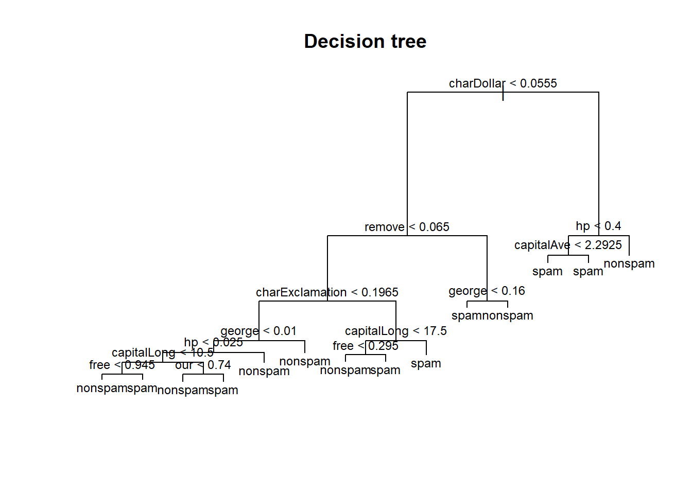
The model may be overtly complicated. Typically, after constructing a decision tree model, we may want to prune the model, by collapsing certain edges, nodes and leaves together without much loss of performance. This is done by iteratively comparing the number of leaf nodes with the model’s performance (by k-fold cross validation within the training set).
cv.prune <- cv.tree(tree.mod, FUN = prune.misclass)
plot(cv.prune$size, cv.prune$dev, pch = 20, col = "red", type = "b",
     main = "Decision tree: Cross validation to find optimal size of tree",
     xlab = "Size of tree", ylab = "Misclassifications")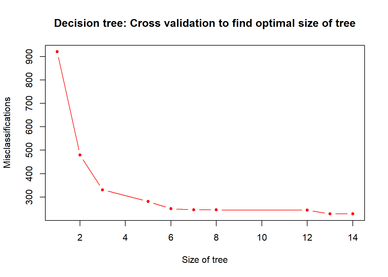
Having 9 leaf nodes may be good (maximising performance while minimising complexity).
best.tree.size <- 9

# pruning (cost-complexity pruning)
pruned.tree.mod <- prune.misclass(tree.mod, best = best.tree.size)

# here's the new tree model
plot(pruned.tree.mod)
title(paste("Pruned decision tree (", best.tree.size, " leaf nodes)",sep = ""))
text(pruned.tree.mod, cex = 0.75)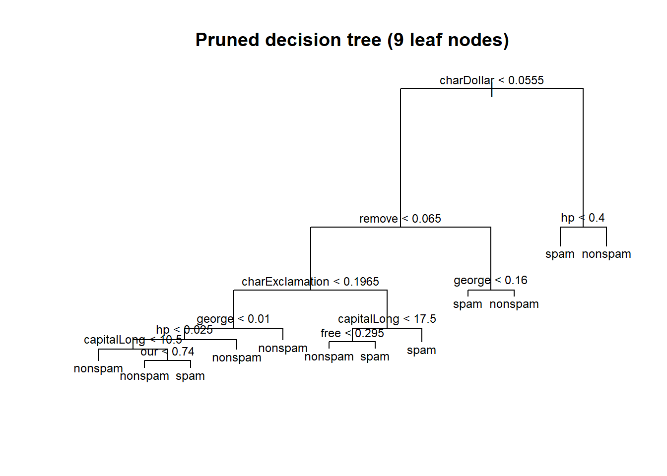
Now with our new model, let’s make some predictions on the testing data.
tree.pred <- predict(pruned.tree.mod,
                     subset(spam.test, select = -type),
                     type = "class")

# confusion matrix
# rows are the predicted classes
# columns are the actual classes
print(tree.pred.results <- table(tree.pred, spam.test$type))
##
## tree.pred nonspam spam
##   nonspam    1325  120
##   spam         83  773

# What is the accuracy of our tree model?
print(tree.accuracy <- (tree.pred.results[1,1] + tree.pred.results[2,2]) / sum(tree.pred.results))
## [1] 0.9117775
Our decision tree model is able to predict spam vs. nonspam emails with about 91.18% accuracy. We will make comparisons of accuracies with other models later.
Bagging
Next, we turn our attention to the bagging model. Recall that bagging, a.k.a. bootstrap aggregating, is the process of sampling (with replacement), samples from the training data. Each of these subsets are known as bags, and we construct individual decision tree models using each of these bags. Finally, to make a classification prediction, we use the majority vote from the ensemble of decision tree models.
bg.mod<-randomForest(type ~ ., data = spam.train,
                     mtry = num.var - 1, # try all variables at each split, except the response variable
                     ntree = 300,
                     proximity = TRUE,
                     importance = TRUE)
In the bagging, and also the random forest model, there are often only two hyperparameters that we are interested in: mtry, which is the number of variables to try from for each tree and at each split, and ntree, the number of trees in the ensemble. Tuning the number of trees is relatively easy by looking at the out-of-bag (OOB) error estimate of the ensemble at each step of the way. For more details, refer to the slides. We set proximity = TRUE and importance = TRUE, in order to get some form of visualization of the model, and the variable importances respectively.
plot(bg.mod$err.rate[,1], type = "l", lwd = 3, col = "blue",
     main = "Bagging: OOB estimate of error rate",
     xlab = "Number of Trees", ylab = "OOB error rate")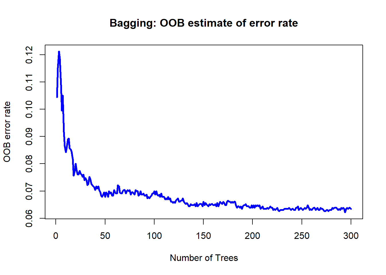
Here, 300 trees seems more than sufficient. One advantage of bagging and random forest models is that they provide a way of doing feature or variable selection, by considering the importance of each variable in the model. For exact details on how these importance measures are defined, refer to the slides.
varImpPlot(bg.mod,
           main = "Bagging: Variable importance")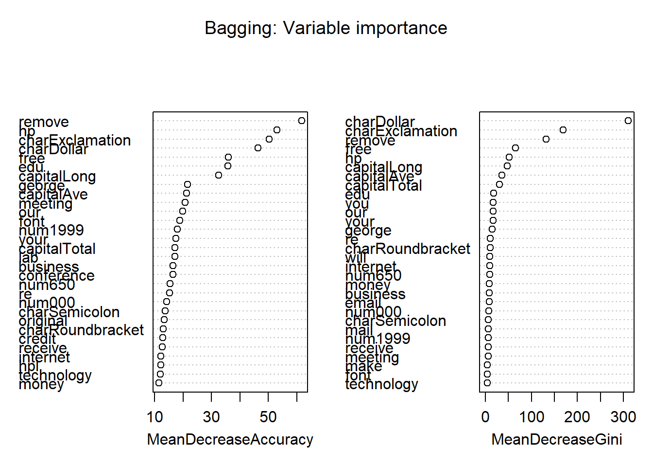
In addition, we can visualize the classification done by the model using a multidimensional plot on the proximity matrix. The green samples in the figure represent nonspams, while the red samples are spams.
MDSplot(bg.mod,
        fac = spam.train$type,
        palette = c("green","red"),
        main = "Bagging: MDS")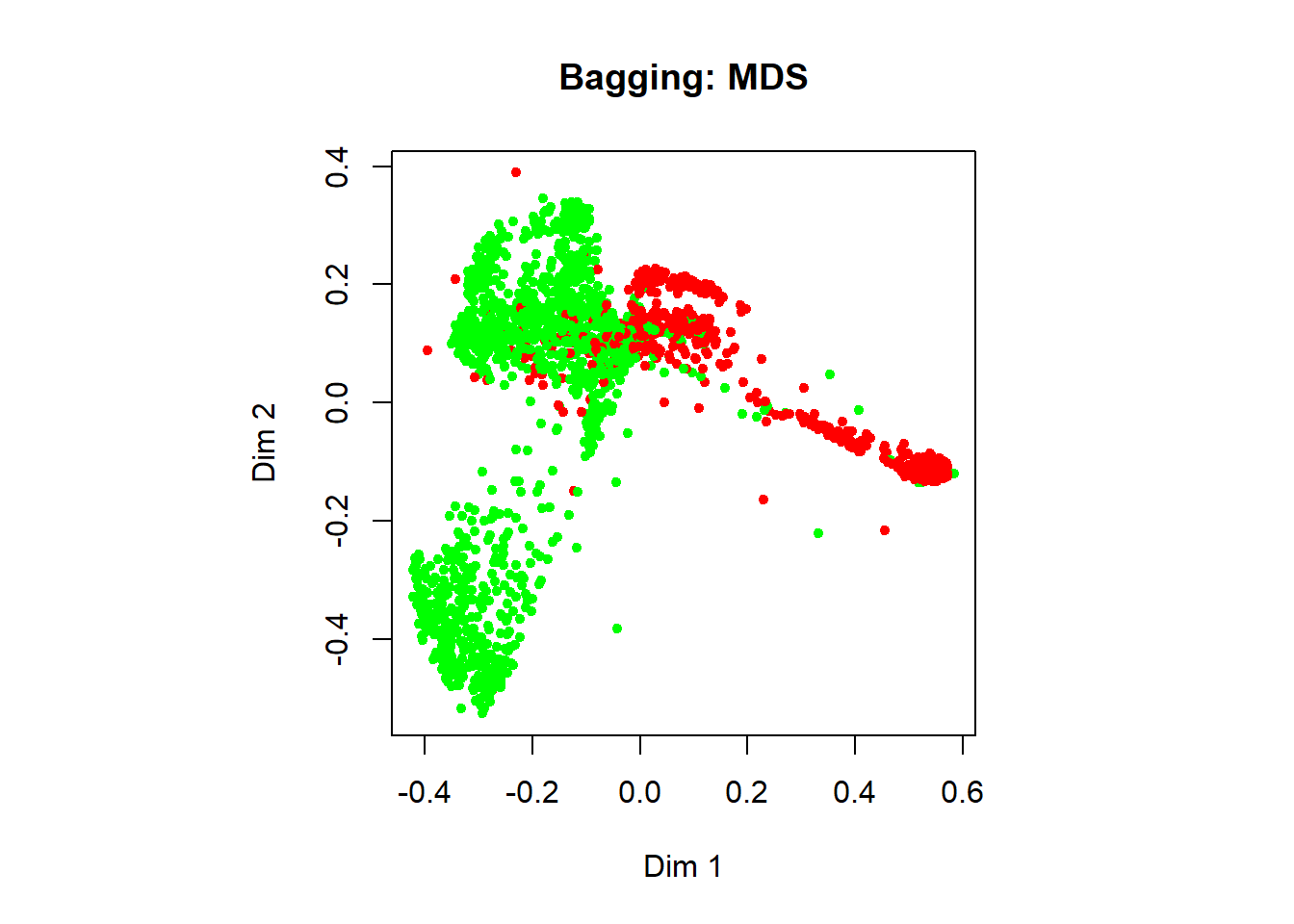
Finally, let’s make some predictions on the testing data:
bg.pred <- predict(bg.mod,
                   subset(spam.test, select = -type),
                   type = "class")

# confusion matrix
# rows are the predicted classes
# columns are the actual classes
print(bg.pred.results <- table(bg.pred, spam.test$type))
##
## bg.pred   nonspam spam
##   nonspam    1358   78
##   spam         50  815

# what is the accuracy of our bagging model?
print(bg.accuracy <- sum(diag((bg.pred.results))) / sum(bg.pred.results))
## [1] 0.944372
Our bagging model predicts whether an email is spam or not with about 94.44% accuracy.
Random Forest
The only difference between the bagging model and random forest model is that the latter uses chooses only from a subset of variables to split on at each node of each tree. In other words, only the mtry argument differs between bagging and random forest.
rf.mod <- randomForest(type ~ ., data = spam.train,
                       mtry = floor(sqrt(num.var - 1)), # 7; only difference from bagging is here
                       ntree = 300,
                       proximity = TRUE,
                       importance = TRUE)

# Out-of-bag (OOB) error rate as a function of num. of trees:
plot(rf.mod$err.rate[,1], type = "l", lwd = 3, col = "blue",
     main = "Random forest: OOB estimate of error rate",
     xlab = "Number of Trees", ylab = "OOB error rate")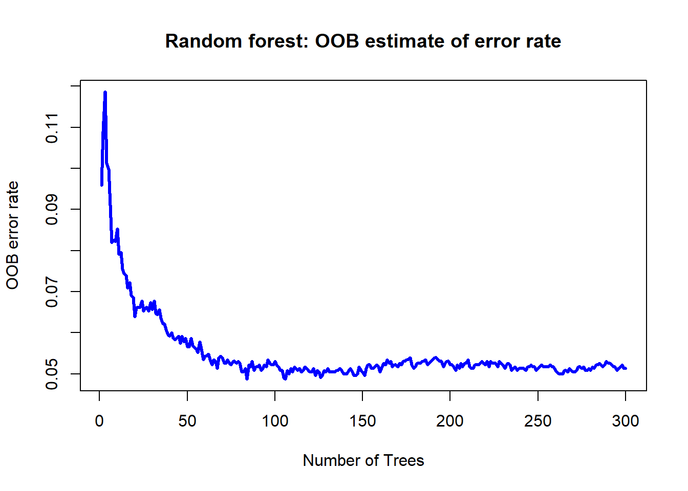
Besides tuning the ntree hyperparameter, we might also be interested in tuning the mtry hyperparameter in random forest. The random forest model may be built using the mtry value that minimises the OOB error.
tuneRF(subset(spam.train, select = -type),
       spam.train$type,
       ntreeTry = 100)
## mtry = 7  OOB error = 5.65%
## Searching left ...
## mtry = 4     OOB error = 5.39%
## 0.04615385 0.05
## Searching right ...
## mtry = 14    OOB error = 5.52%
## 0.02307692 0.05
##        mtry   OOBError
## 4.OOB     4 0.05391304
## 7.OOB     7 0.05652174
## 14.OOB   14 0.05521739
title("Random forest: Tuning the mtry hyperparameter")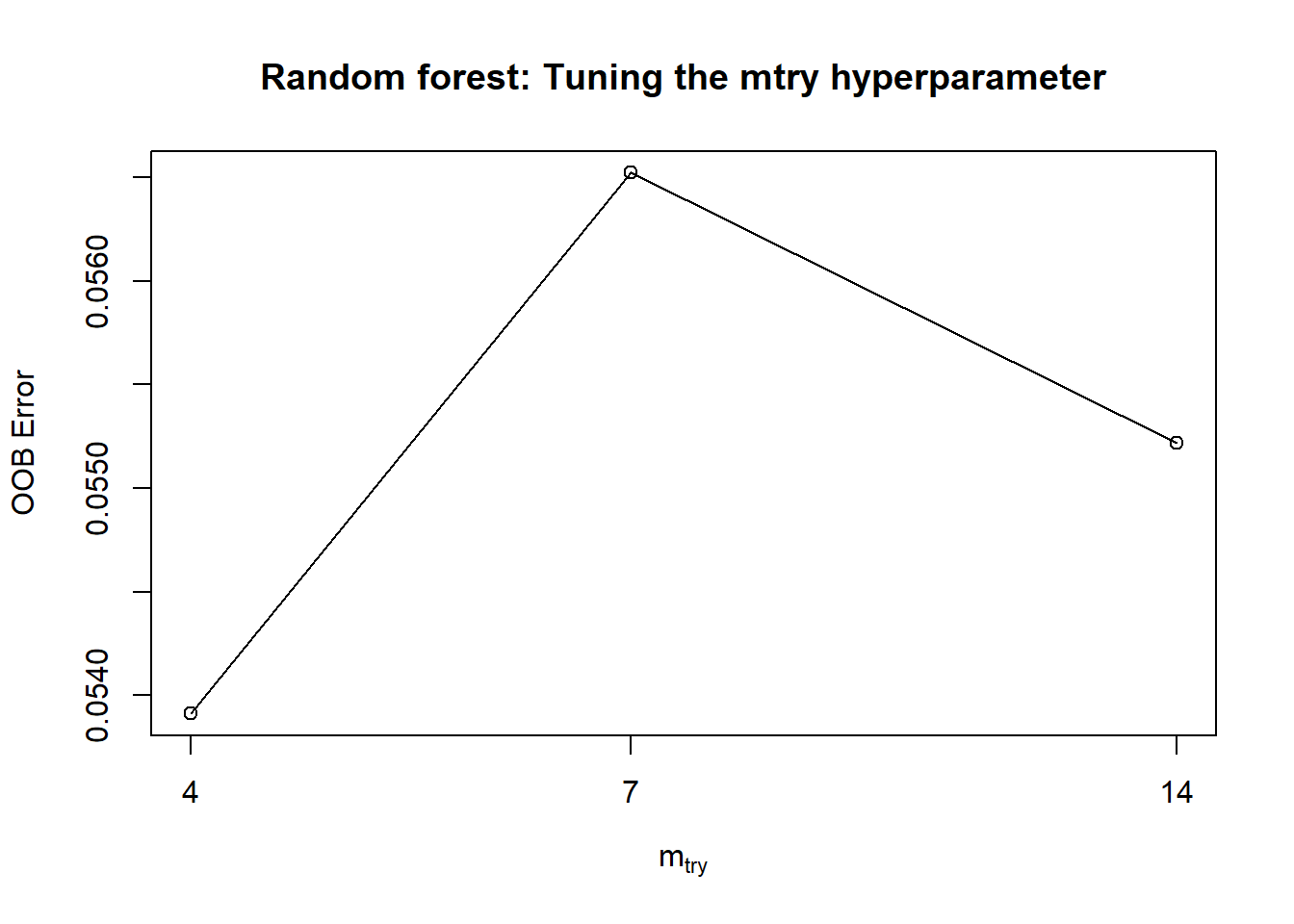
# variable importance
varImpPlot(rf.mod,
           main = "Random forest: Variable importance")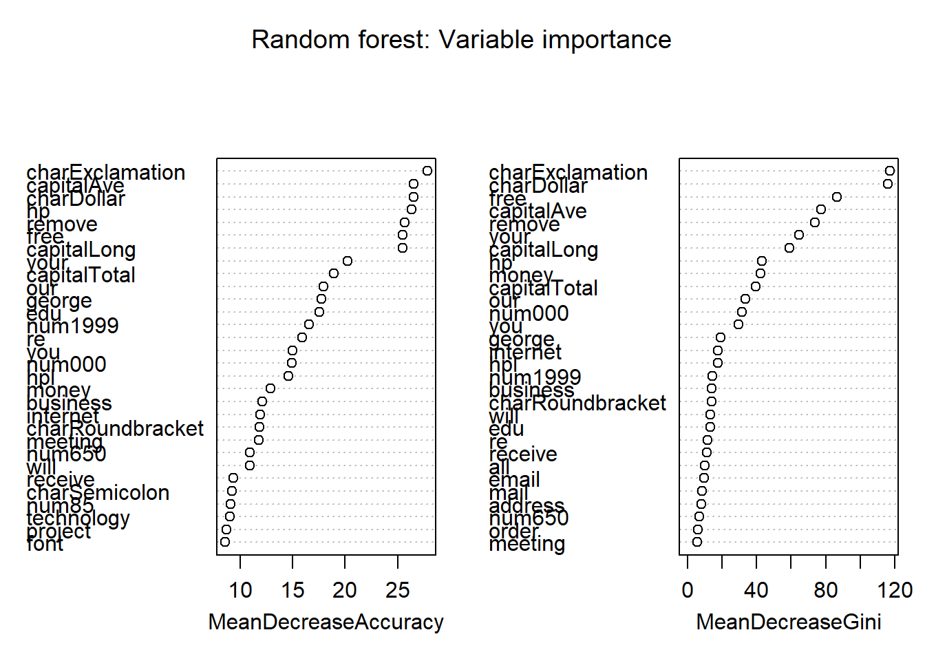
# multidimensional scaling plot
# green samples are non-spam,
# red samples are spam
MDSplot(rf.mod,
        fac = spam.train$type,
        palette = c("green","red"),
        main = "Random forest: MDS")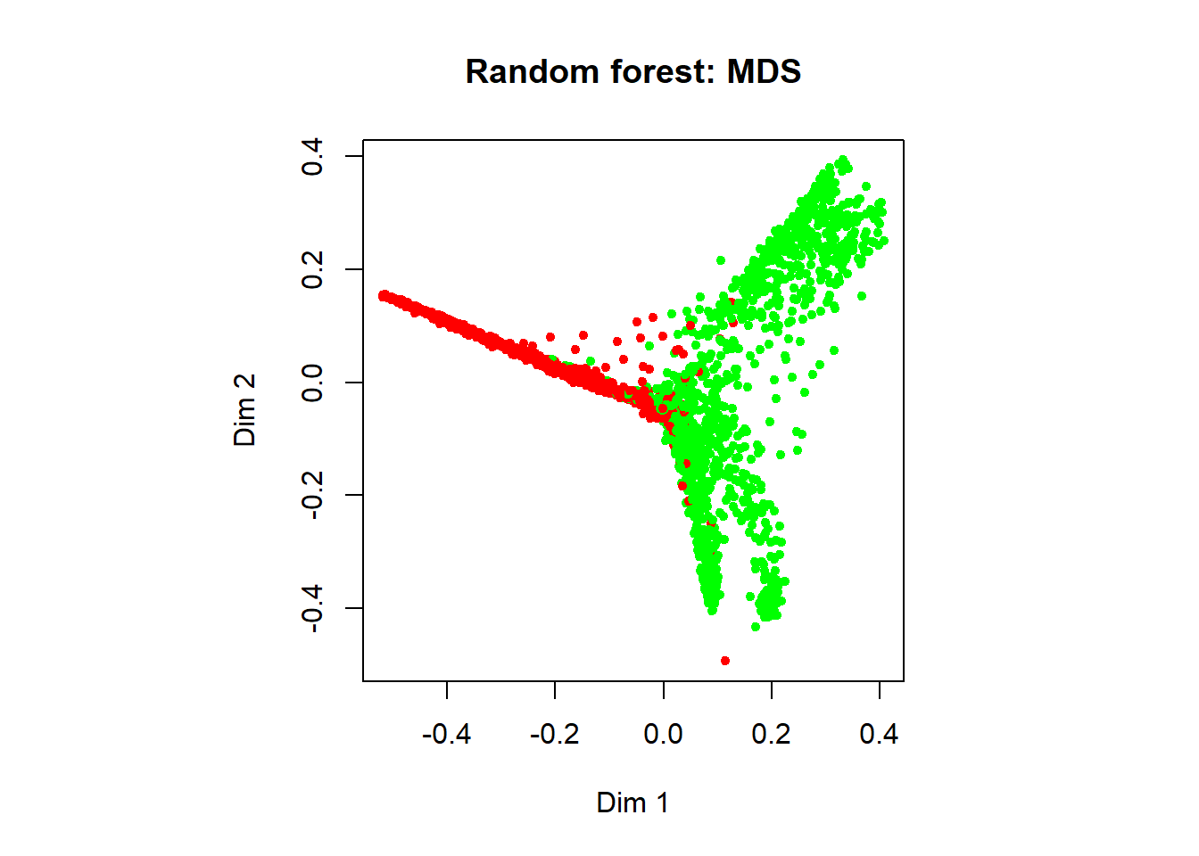
# now, let's make some predictions
rf.pred <- predict(rf.mod,
                   subset(spam.test,select = -type),
                   type="class")

# confusion matrix
print(rf.pred.results <- table(rf.pred, spam.test$type))
##
## rf.pred   nonspam spam
##   nonspam    1372   80
##   spam         36  813

# Accuracy of our RF model:
print(rf.accuracy <- sum(diag((rf.pred.results))) / sum(rf.pred.results))
## [1] 0.9495871
Our random forest model predicts whether an email is spam or not with about 94.96% accuracy.
Visualization of performances
Let’s go ahead and make some comparisons on the performances of our model. For comparison sake, let’s also construct a logistic regression model.
log.mod <- glm(type ~ . , data = spam.train,
             family = binomial(link = logit))
## Warning: glm.fit: fitted probabilities numerically 0 or 1 occurred

# predictions
log.pred.prob <- predict(log.mod,
                         subset(spam.test, select = -type),
                         type = "response")
log.pred.class <- factor(sapply(log.pred.prob,
                                FUN = function(x){
                                        if(x >= 0.5) return("spam")
                                        else return("nonspam")
                                }))

# confusion matrix
log.pred.results <- table(log.pred.class, spam.test$type)

# Accuracy of logistic regression model:
print(log.accuracy <- sum(diag((log.pred.results))) / sum(log.pred.results))
## [1] 0.9126467
Now, let’s compare the performances, considering first the model accuracies.
barplot(c(tree.accuracy,
          bg.accuracy,
          rf.accuracy,
          log.accuracy),
        main="Accuracies of various models",
        names.arg=c("Tree","Bagging","RF", "Logistic"))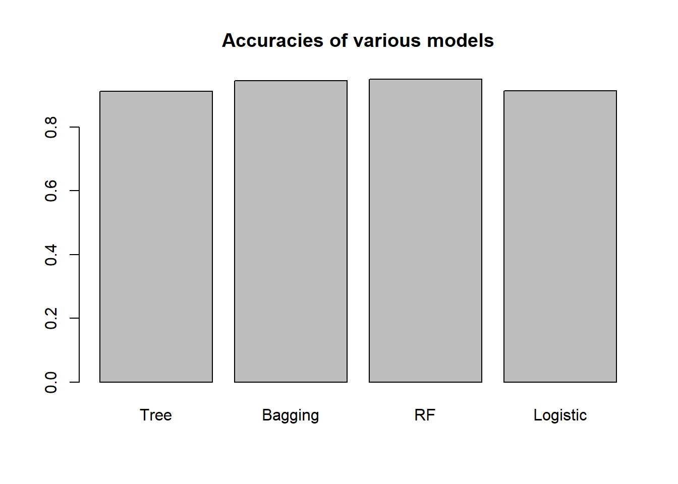
We can see here that the ensemble models (bagging and random forest) outperforms the single decision tree, and also the logistic regression model. It turns out here that the bagging and the random forest models have about the same classification performance. Understanding the rationale of random subspace sampling (refer to slides) should allow us to appreciate the potential improvement of random forest over the bagging model.
Finally, let’s plot the ROC curves of the various models. The ROC is only valid for models that give probabilistic output.
bg.pred.prob <- predict(bg.mod ,
                        subset(spam.test, select = -type),
                        type = "prob")

rf.pred.prob <- predict(rf.mod ,
                        subset(spam.test, select = -type),
                        type = "prob")

plot.roc(spam.test$type,
         bg.pred.prob[,1], col = "blue",
         lwd = 3, print.auc = TRUE, print.auc.y = 0.3,
         main = "ROC-AUC of various models")
## Setting levels: control = nonspam, case = spam
## Setting direction: controls > cases

plot.roc(spam.test$type,
         rf.pred.prob[,1], col = "green",
         lwd = 3, print.auc = TRUE, print.auc.y = 0.2,
         add = TRUE)
## Setting levels: control = nonspam, case = spam
## Setting direction: controls > cases

plot.roc(spam.test$type,
         log.pred.prob, col = "red",
         lwd = 3, print.auc = TRUE, print.auc.y = 0.1,
         add = TRUE)
## Setting levels: control = nonspam, case = spam
## Setting direction: controls < cases

legend(x = 0.6, y = 0.8, legend = c("Bagging",
                                    "Random forest",
                                    "Logistic regression"),
       col = c("blue", "green", "red"), lwd = 1)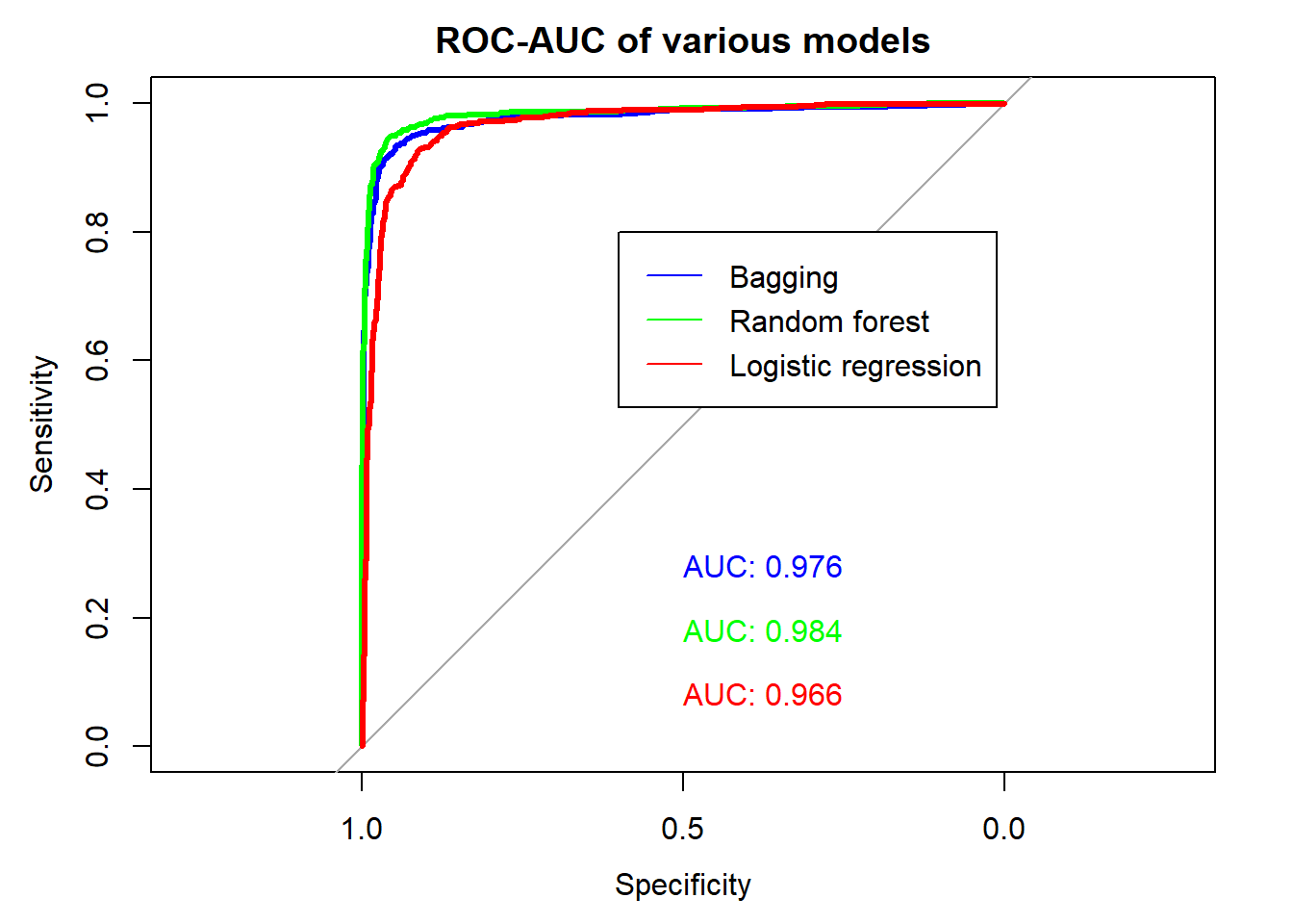
Tree-based methods for regression
In the following section, we will consider the use of tree-based methods for regression. The materials that follows are analogous to that above, if not the similar.
Preparation
library(tree)
library(randomForest)

data(imports85)
imp <- imports85

# The following data preprocessing steps on
# the imports85 dataset are suggested by
# the authors of the randomForest package
# look at
# > ?imports85
imp <- imp[,-2]  # Too many NAs in normalizedLosses.
imp <- imp[complete.cases(imp), ]
# ## Drop empty levels for factors
imp[] <- lapply(imp, function(x) if (is.factor(x)) x[, drop=TRUE] else x)

# Also removing the numOfCylinders and fuelSystem
# variables due to sparsity of data
# to see this, run the following lines:
# > table(imp$numOfCylinders)
# > table(imp$fuelSystem)
# This additional step is only necessary because we will be
# making comparisons between the tree-based models
# and linear regression, and linear regression cannot
# handle sparse data well
imp <- subset(imp, select = -c(numOfCylinders,fuelSystem))

# also removing the make variable
imp <- subset(imp, select = -make)

# Preparation for cross validation:
# split the dataset into 2 halves,
# 96 samples for training and 97 for testing
num.samples <- nrow(imp) # 193
num.train   <- round(num.samples / 2) # 96
num.test    <- num.samples - num.train # 97
num.var     <- ncol(imp) # 25

# set up the indices
set.seed(150715)
idx       <- sample(1:num.samples)
train.idx <- idx[seq(num.train)]
test.idx  <- setdiff(idx,train.idx)

# subset the data
imp.train <- imp[train.idx,]
imp.test  <- imp[test.idx,]

str(imp.train)
## 'data.frame':    96 obs. of  22 variables:
##  $ symboling       : int  3 1 1 1 3 1 1 1 0 2 ...
##  $ fuelType        : Factor w/ 2 levels "diesel","gas": 2 2 2 2 2 2 2 1 2 2 ...
##  $ aspiration      : Factor w/ 2 levels "std","turbo": 1 1 1 1 2 1 1 1 1 1 ...
##  $ numOfDoors      : Factor w/ 2 levels "four","two": 2 1 2 2 2 1 2 2 1 2 ...
##  $ bodyStyle       : Factor w/ 5 levels "convertible",..: 1 4 4 3 3 3 3 4 4 4 ...
##  $ driveWheels     : Factor w/ 3 levels "4wd","fwd","rwd": 2 2 2 2 2 2 2 2 3 2 ...
##  $ engineLocation  : Factor w/ 2 levels "front","rear": 1 1 1 1 1 1 1 1 1 1 ...
##  $ wheelBase       : num  94.5 93.1 94.5 93.7 95.9 93.7 93.1 94.5 113 99.8 ...
##  $ length          : num  159 167 165 157 173 ...
##  $ width           : num  64.2 64.2 63.8 63.8 66.3 63.8 64.2 63.8 69.6 66.3 ...
##  $ height          : num  55.6 54.1 54.5 50.8 50.2 50.6 54.1 54.5 52.8 53.1 ...
##  $ curbWeight      : int  2254 1945 1918 1876 2921 1967 1905 2017 4066 2507 ...
##  $ engineType      : Factor w/ 5 levels "dohc","l","ohc",..: 3 3 3 3 3 3 3 3 1 3 ...
##  $ engineSize      : int  109 91 97 90 156 90 91 103 258 136 ...
##  $ bore            : num  3.19 3.03 3.15 2.97 3.59 2.97 3.03 2.99 3.63 3.19 ...
##  $ stroke          : num  3.4 3.15 3.29 3.23 3.86 3.23 3.15 3.47 4.17 3.4 ...
##  $ compressionRatio: num  8.5 9 9.4 9.41 7 9.4 9 21.9 8.1 8.5 ...
##  $ horsepower      : int  90 68 69 68 145 68 68 55 176 110 ...
##  $ peakRpm         : int  5500 5000 5200 5500 5000 5500 5000 4800 4750 5500 ...
##  $ cityMpg         : int  24 31 31 37 19 31 31 45 15 19 ...
##  $ highwayMpg      : int  29 38 37 41 24 38 38 50 19 25 ...
##  $ price           : int  11595 6695 6649 5572 14869 6229 6795 7099 35550 15250 ...
str(imp.test)
## 'data.frame':    97 obs. of  22 variables:
##  $ symboling       : int  -1 0 1 0 3 0 0 3 2 2 ...
##  $ fuelType        : Factor w/ 2 levels "diesel","gas": 2 2 2 2 2 2 2 2 2 2 ...
##  $ aspiration      : Factor w/ 2 levels "std","turbo": 1 1 2 1 2 1 1 1 1 1 ...
##  $ numOfDoors      : Factor w/ 2 levels "four","two": 1 1 2 1 2 2 1 2 2 1 ...
##  $ bodyStyle       : Factor w/ 5 levels "convertible",..: 4 3 3 4 3 3 4 3 3 4 ...
##  $ driveWheels     : Factor w/ 3 levels "4wd","fwd","rwd": 2 2 3 1 2 2 2 2 1 2 ...
##  $ engineLocation  : Factor w/ 2 levels "front","rear": 1 1 1 1 1 1 1 1 1 1 ...
##  $ wheelBase       : num  102.4 97.2 102.7 97 95.9 ...
##  $ length          : num  176 173 178 172 173 ...
##  $ width           : num  66.5 65.2 68 65.4 66.3 65.2 65.2 66.5 63.8 66.5 ...
##  $ height          : num  54.9 54.7 54.8 54.3 50.2 53.3 54.1 56.1 55.7 56.1 ...
##  $ curbWeight      : int  2414 2324 2910 2385 2811 2236 2304 2658 2240 2758 ...
##  $ engineType      : Factor w/ 5 levels "dohc","l","ohc",..: 3 3 3 4 3 3 3 3 4 3 ...
##  $ engineSize      : int  122 120 140 108 156 110 110 121 108 121 ...
##  $ bore            : num  3.31 3.33 3.78 3.62 3.6 3.15 3.15 3.54 3.62 3.54 ...
##  $ stroke          : num  3.54 3.47 3.12 2.64 3.9 3.58 3.58 3.07 2.64 3.07 ...
##  $ compressionRatio: num  8.7 8.5 8 9 7 9 9 9.31 8.7 9.3 ...
##  $ horsepower      : int  92 97 175 82 145 86 86 110 73 110 ...
##  $ peakRpm         : int  4200 5200 5000 4800 5000 5800 5800 5250 4400 5250 ...
##  $ cityMpg         : int  27 27 19 24 19 27 27 21 26 21 ...
##  $ highwayMpg      : int  32 34 24 25 24 33 33 28 31 28 ...
##  $ price           : int  10898 8949 16503 9233 12964 7895 8845 11850 7603 15510 ...

# take a quick look
hist(imp.train$price)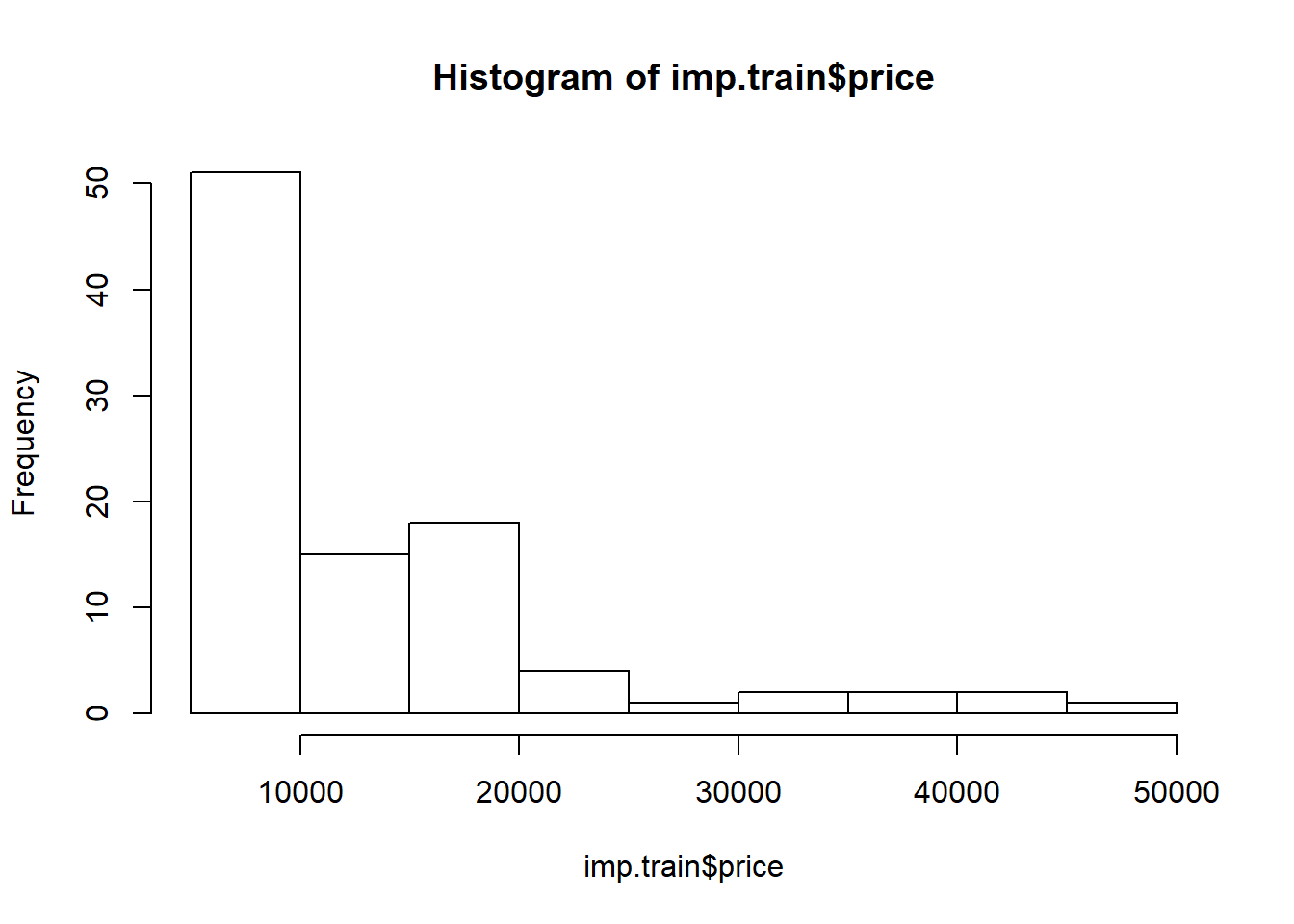
hist(imp.test$price)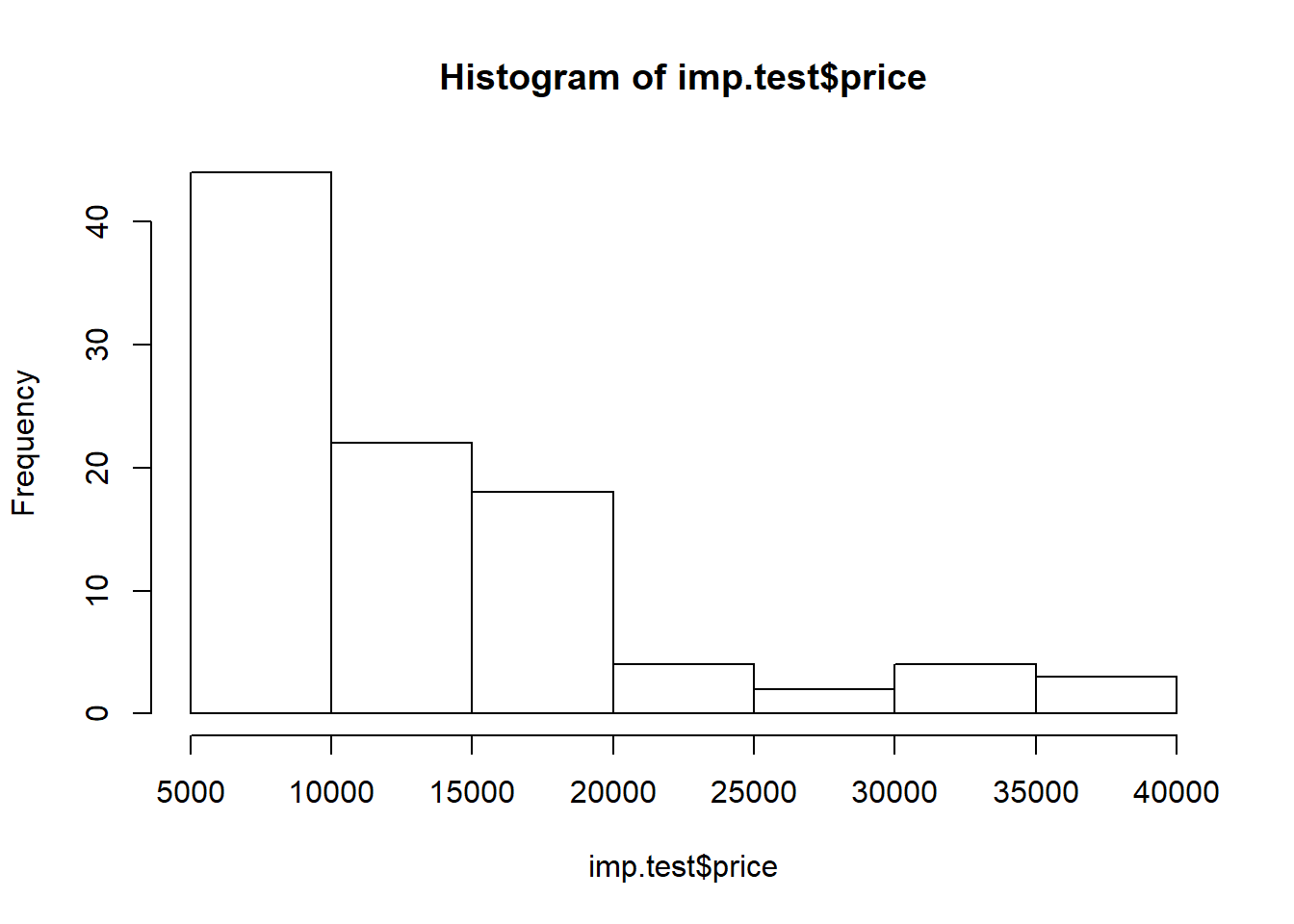
We will be predicting the price of imported automobiles in this example. While tree-based methods are scale-invariant with respect to predictor variables, this is not true for the response variable. Hence, let’s take a log-transformation on price here.
imp.train$price <- log(imp.train$price)
imp.test$price <- log(imp.test$price)

# take a look again
hist(imp.train$price)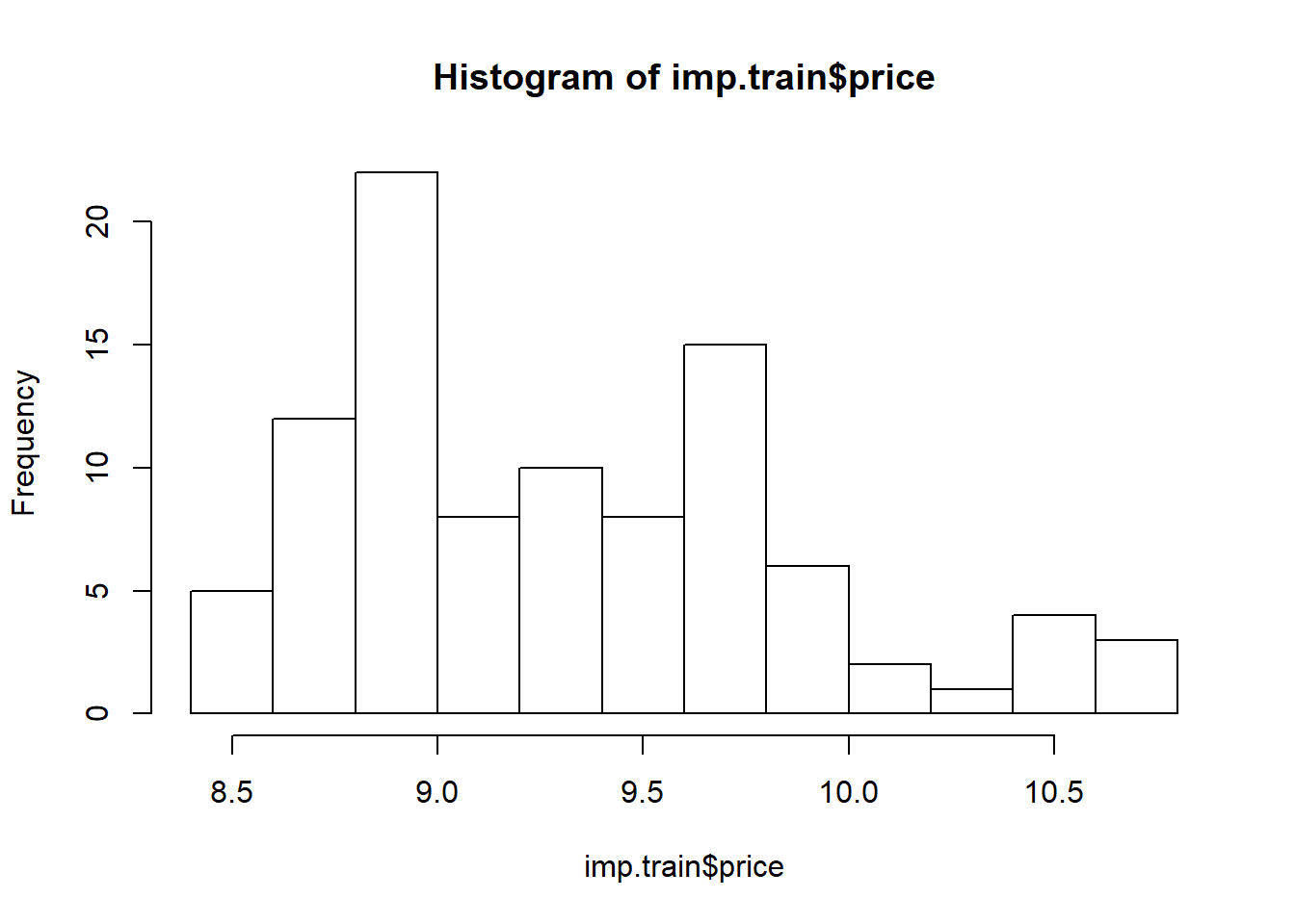
hist(imp.test$price)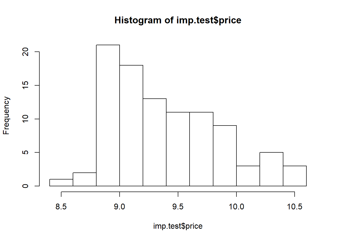
Decision tree
Done with the preparation, let’s begin with decision trees.
# Construct decision tree model
tree.mod <- tree(price ~ ., data = imp.train)

# here's how the model looks like
plot(tree.mod)
title("Decision tree")
text(tree.mod, cex = 0.75)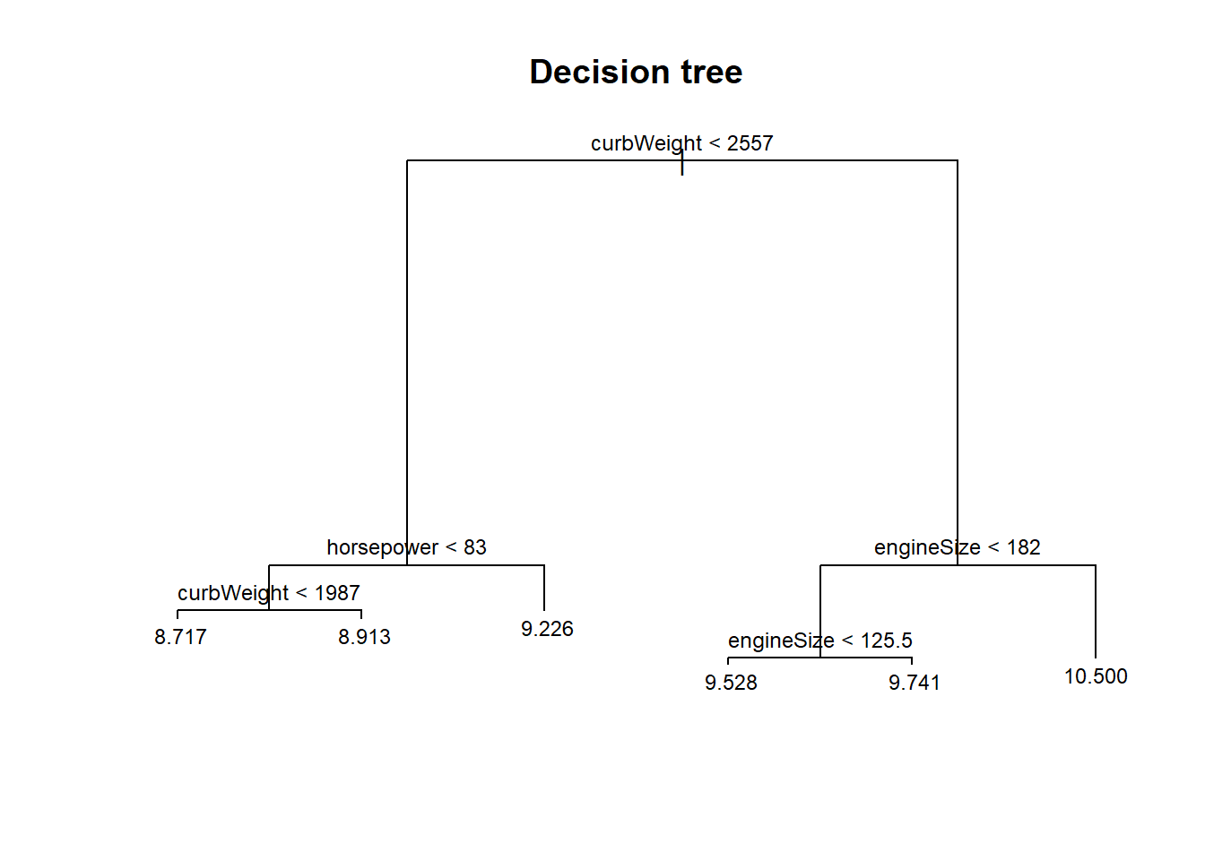
# let's see if our decision tree requires pruning
cv.prune <- cv.tree(tree.mod, FUN = prune.tree)
plot(cv.prune$size, cv.prune$dev, pch = 20, col = "red", type = "b",
     main = "Cross validation to find optimal size of tree",
     xlab = "Size of tree", ylab = "Mean squared error")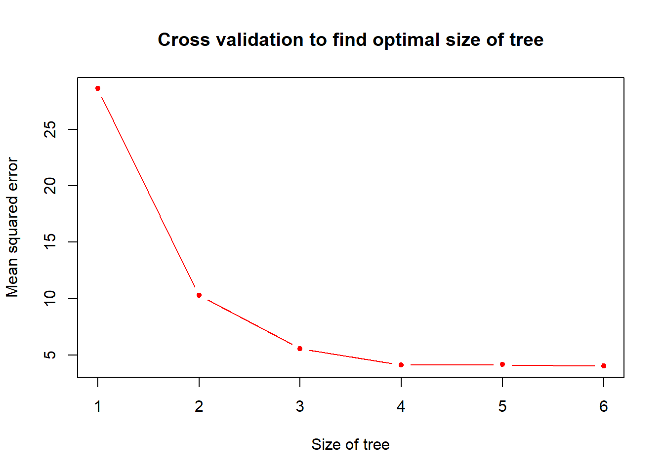
# looks fine

# now let's make some predictions
tree.pred <- predict(tree.mod,
                     subset(imp.test,select = -price),
                     type = "vector")

# Comparing our predictions with the test data:
plot(tree.pred, imp.test$price, main = "Decision tree: Actual vs. predicted")
abline(a = 0, b = 1) # A prediction with zero error will lie on the y = x line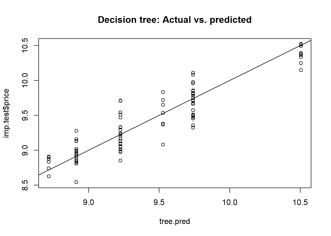
# What is the MSE of our model?
print(tree.mse <- mean((tree.pred - imp.test$price) ** 2))
## [1] 0.0391897
Our decision tree model predicts the price of imported automobiles with a mean squared error of 0.0392. As with the previous section, we will make comparsions on model performances later.
Bagging
Next, bagging.
bg.mod<-randomForest(price ~ ., data = imp.train,
                     mtry = num.var - 1, # try all variables at each split, except the response variable
                     ntree = 300,
                     importance = TRUE)

# Out-of-bag (OOB) error rate as a function of num. of trees
# here, the error is the mean squared error,
# not classification error
plot(bg.mod$mse, type = "l", lwd = 3, col = "blue",
     main = "Bagging: OOB estimate of error rate",
     xlab = "Number of Trees", ylab = "OOB error rate")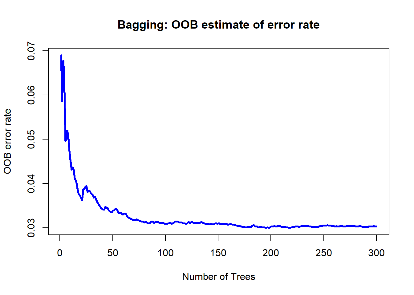
# variable importance
varImpPlot(bg.mod,
           main = "Bagging: Variable importance")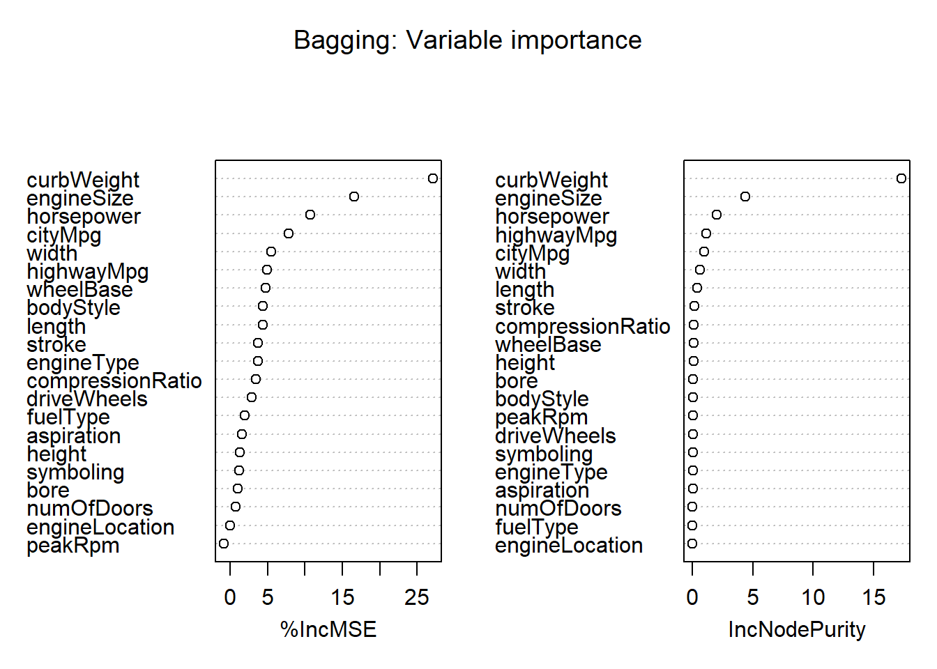
# let's make some predictions
bg.pred <- predict(bg.mod,
                   subset(imp.test,select = -price))

# Comparing our predictions with test data:
plot(bg.pred,imp.test$price, main = "Bagging: Actual vs. predicted")
abline(a = 0, b = 1)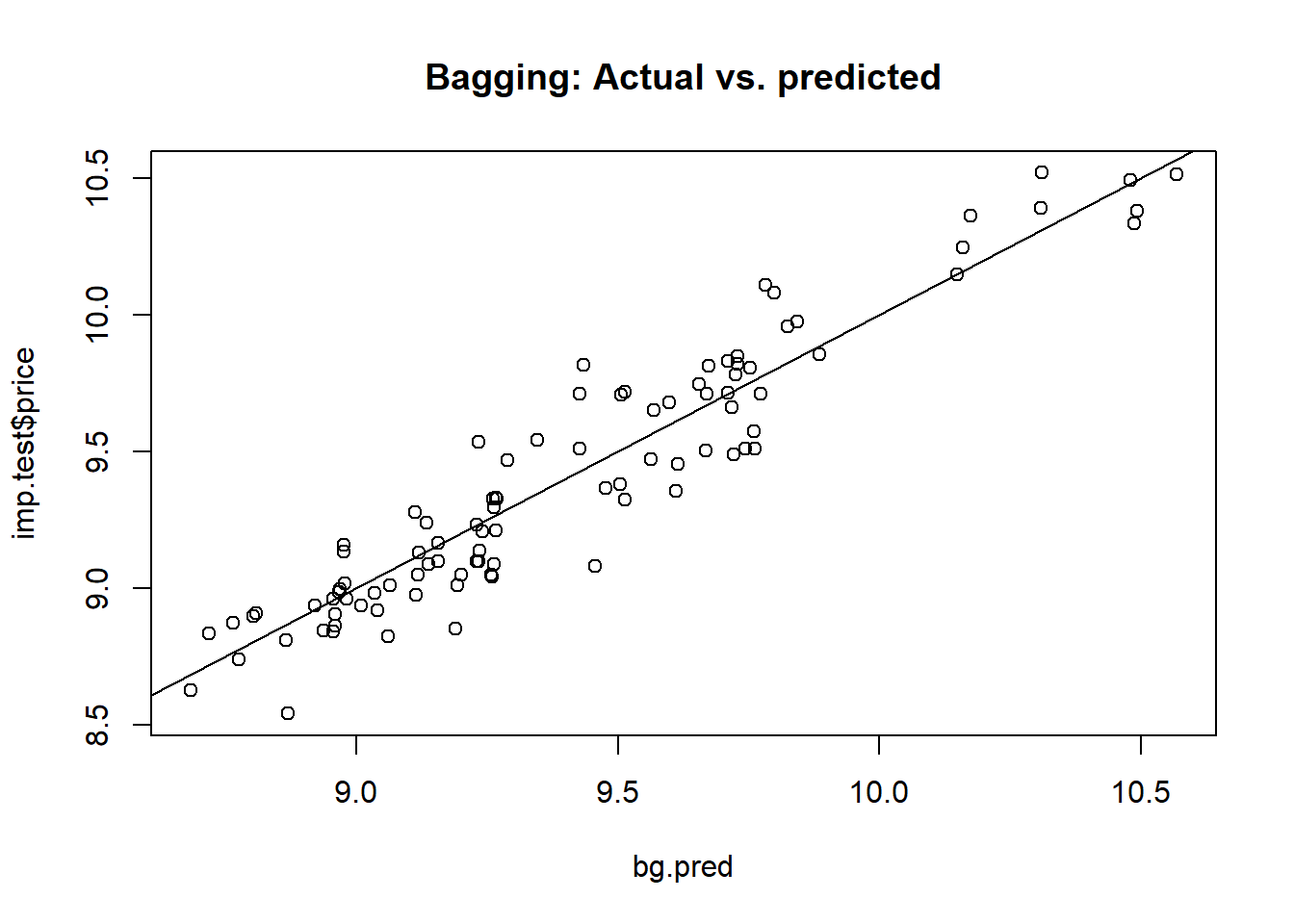
# MSE of bagged model
print(bg.mse <- mean((bg.pred - imp.test$price) ** 2))
## [1] 0.02298332
Our bagging model predicts the price of imported automobiles with a mean squared error of 0.023.
Random forest
Finally, the random forest model.
rf.mod<-randomForest(price ~ ., data = imp.train,
                     mtry = floor((num.var - 1) / 3), # 7; only difference from bagging is here
                     ntree = 300,
                     importance = TRUE)

# Out-of-bag (OOB) error rate as a function of num. of trees
plot(rf.mod$mse, type = "l", lwd = 3, col = "blue",
     main = "Random forest: OOB estimate of error rate",
     xlab = "Number of Trees", ylab = "OOB error rate")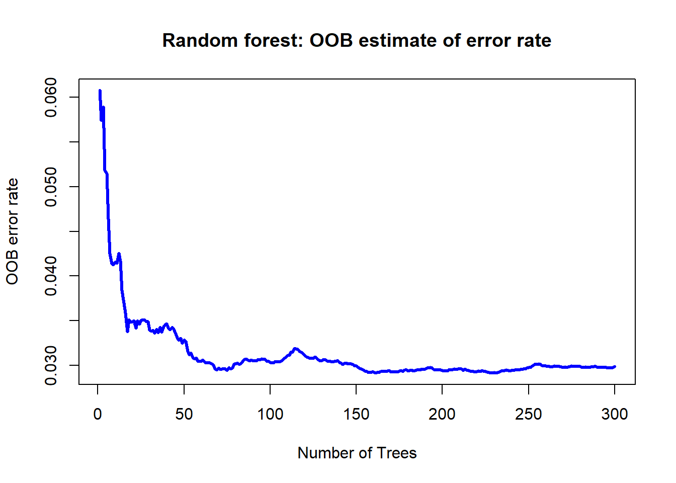
# tuning the mtry hyperparameter:
# model may be rebuilt if desired
tuneRF(subset(imp.train, select = -price),
       imp.train$price,
       ntreetry = 100)
## mtry = 7  OOB error = 0.03033217
## Searching left ...
## mtry = 4     OOB error = 0.03732523
## -0.2305491 0.05
## Searching right ...
## mtry = 14    OOB error = 0.0289063
## 0.04700843 0.05
##    mtry   OOBError
## 4     4 0.03732523
## 7     7 0.03033217
## 14   14 0.02890630
title("Random forest: Tuning the mtry hyperparameter")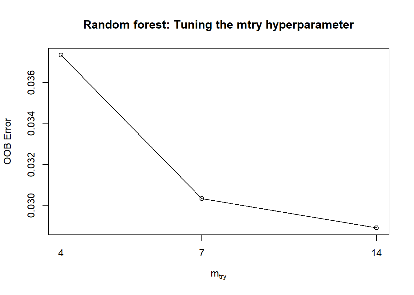
# variable importance
varImpPlot(rf.mod,
           main = "Random forest: Variable importance")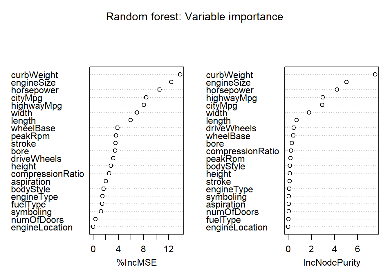
# let's make some predictions
rf.pred <- predict(rf.mod,
                   subset(imp.test, select = -price))

# Comparing our predictions with test data:
plot(rf.pred, imp.test$price, main = "Random forest: Actual vs. predicted")
abline(a = 0, b = 1)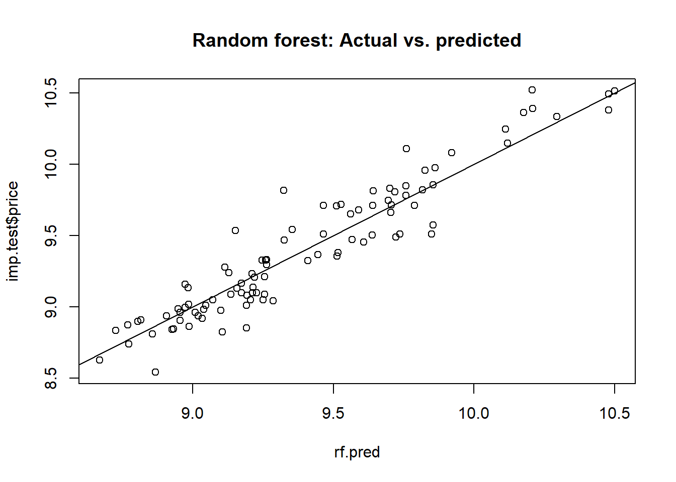
# MSE of RF model
print(rf.mse <- mean((rf.pred - imp.test$price) ** 2))
## [1] 0.02317156
Our random forest model incurs a mean squared error of 0.0232 for the prediction of imported automobile prices
Visualization of performances
For comparison purposes, let’s also construct a ordinary least squares (linear regression) model.
ols.mod <- lm(price ~ ., data = imp.train)

# predictions
ols.pred <- predict(ols.mod,
                   subset(imp.test, select = -price))

# comparisons with test data:
plot(ols.pred, imp.test$price, main = "OLS: Actual vs. predicted")
abline(a = 0, b = 1)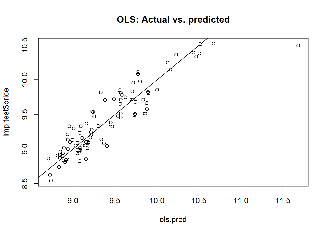
# MSE
print(ols.mse <- mean((ols.pred-imp.test$price) ** 2))
## [1] 0.04616828
Now, let’s compare their performances.
# Comparing MSEs of various models:
barplot(c(tree.mse,
          bg.mse,
          rf.mse,
          ols.mse),
        main = "Mean squared errors of various models",
        names.arg = c("Tree", "Bagging", "RF", "OLS"))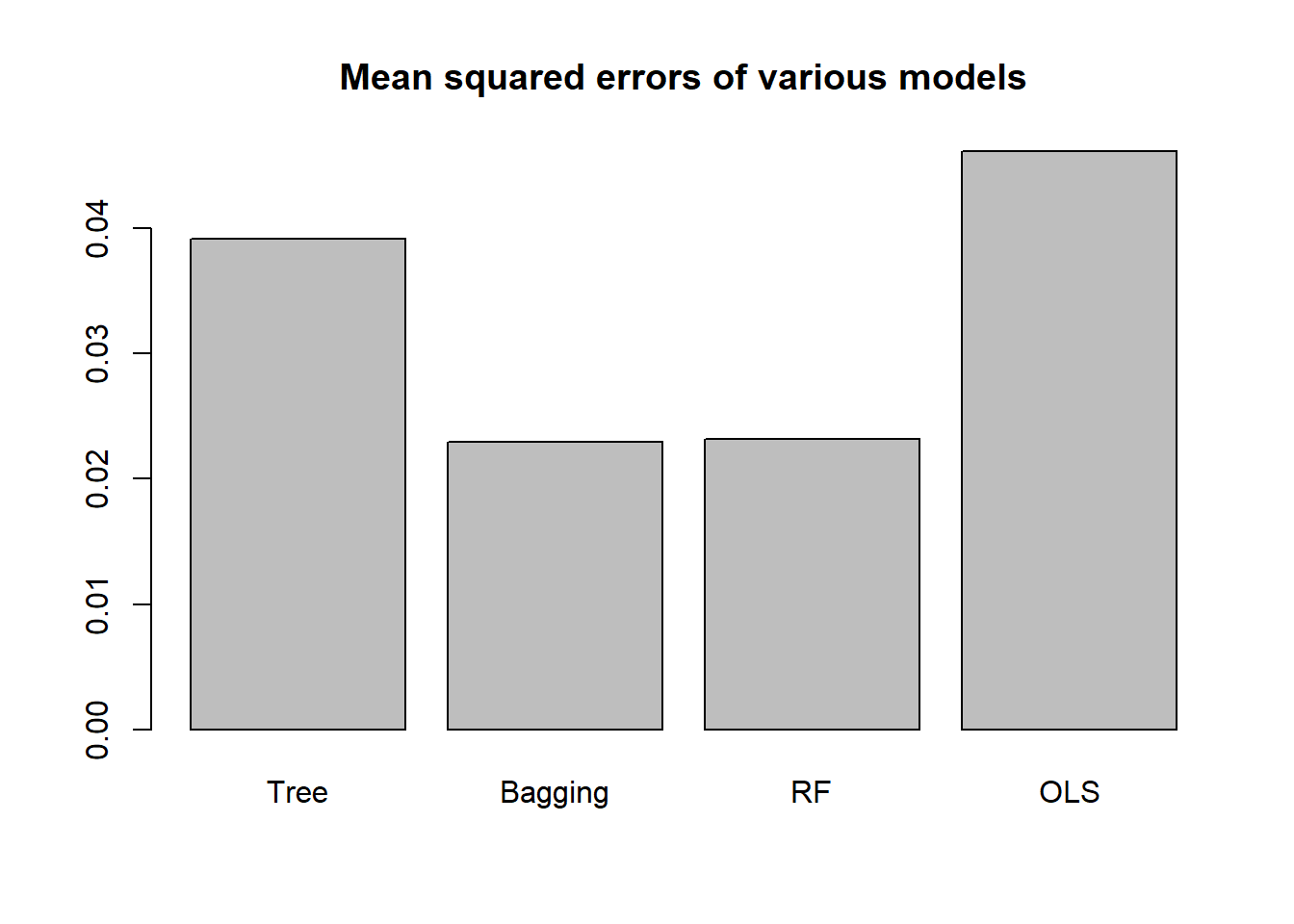
Our top performer here is the random forest model, followed by the bagging model.