Introduction
In this post, I would like to talk about modern portfolio theory (MPT), a key topic in finance. The first couple of lines in the MPT Wikipedia article explains it very well:
(MPT) is a mathematical framework for assembling a portfolio of assets such that the expected return is maximized for a given level of risk. It is a formalization and extension of diversification in investing, the idea that owning different kinds of financial assets is less risky than owning only one type. Its key insight is that an asset’s risk and return should not be assessed by itself, but by how it contributes to a portfolio’s overall risk and return. It uses the variance of asset prices as a proxy for risk.
The objective of the MPT is to simultaneously maximise the returns of a portfolio, while at the same time, minimise the risk of the portfolio. Generally, we all know that higher returns come with higher risk, and therefore the dual goals of maximising returns while minimising risk are at odds with each other. After all, why would an investor place himself in a riskier position without any due reward or risk premium? It wouldn’t make sense. Note that in this and many statistical finance frameworks, risk is often measured by means of standard deviation of returns, either that of the asset or the portfolio1.
As a “gentle introduction” to MPT, in this post, all you need is the basic understanding of mean, variance, and covariance. I will do the rest by repeatedly applying these three statistics in the context of a portfolio - nothing more, nothing less!
Terminology
Risk premium refers to the difference between the expected return between a risky asset, like a stock, and that of something that basically has no risk, like cash, Treasury Bills or Singapore Savings Bonds. Without any risk premium, there’s no reason to invest in anything other than risk-free assets.
Problem formulation
Suppose there are \(N\) assets with \(R_i, i = 1, ..., N\) denoting the random variables that represent their respective returns in a given time period, and \(\mathbf{R} = (R_1, ..., R_N)^{T}\).
Their returns and risks are respectively
\[ \begin{array}{c} r_i = ER_i \\\ \sigma_i = Var(R_i)\\\ cov(\mathbf{R}) = \Sigma = (\sigma_{ij})_{1 \le i,j \le N} \end{array} \] We can then form a portfolio consisting of the \(N\) assets such that
\[ \begin{array}{c} R_{pf} = w_1R_1 + ... + w_NR_N = w^T\mathbf{R}, \end{array} \]
where \(R_{pf}\) is the return of the portfolio and \(w_i\) is the weight of the \(i\)th asset in the portfolio, with
\[\sum_{i = 1}^{N} w_i = 1\]
In other words, the portfolio is the linear combination of the various assets under consideration. Of course, the question that becomes: how to choose \(\mathbf{w} = (w_1, ..., w_N)^T\) such that expected returns are maximised while minimising risk?
Portfolio weights
A technical point to bring out here is that while \(\sum_{i = 1}^{N} w_i = 1\), there is no constraint on individual \(w_i\) to be non-negative. In fact, a negative \(w_i\) implies a short position in the \(i\)th asset, i.e. short selling. This is in constrast to a long position, i.e. buying the \(i\)th asset. In this post, we will only consider positive \(w_i\) only.
Terminology
Holding a long position in a particular asset simply means buying that particular asset. On the other hand, short selling is where one sells an asset without owning it in the first place. The asset, e.g. a stock, is borrowed from a broker or another customer of the broker. At a later point in time, a stock must then be bought back from the market and then returned to the lender. This closes the short position, and the idea is that if one is able to sell the borrowed stock at a higher price and return it at a lower price, a profit is made.
Portfolio expectation and variance
With this set-up, the expectation and variance of the portfolio would be
\[ER_{pf} = \sum_iw_iER_i = \mathbf{w}^TE\mathbf{R}\] \[Var(R_{pf}) = \sum_iw_i^2\sigma_i^2 + \sum_i\sum_{j\neq i}w_iw_j\sigma_{ij}\] where \(\sigma_{ij}\) is the covariance between the \(i\)th and \(j\)th asset.
Alternatively,
\[Var(R_{pf}) = \sum_i\sum_jw_iw_j\sigma_{ij} = \mathbf{w}_T\Sigma \mathbf{w}\]
The math behind diversification
We all know “not to put our eggs in one basket”, and have a diversified portfolio. Intutitively, we know that if we were to put all our money on a single stock, then we have placed a large bet on that one company. While we could instantly make it big just by having our one stock making it big, loss aversion would dictate that we would rather minimise the risk of losing it all in a single stock.
In this sense, what diversification does to a portfolio is that it minimises risk of the portfolio. While the mean return of a portfolio depends on the mean returns of the individual assets and their respective weights, the risk of the portfolio depends on both the risk of the individual assets, as well as each asset’s relationships with the others, in terms of correlations.
This means that placing a right mix of weights and assets would reduce the risk of the portfolio - a fundamental idea in portfolio theory. Diversification, by way of investing in multiple assets, reduces risks.
Let’s consider two instructive examples.
Starting with two assets
Again, the objective of treating portfolio selection as a statistical problem is to select individual \(w_i\) such that \(ER_{pf}\) is large and \(Var(R_{pf})\) is small. As with our two instructive examples above, we can start solving this problem by first considering \(N = 2\), that is, choosing the weights \(w_i\) between two assets only. Inevitably, we would have
\[ \begin{array}{c} ER_{pf} = \sum_iw_iER_i = w_1ER_1 + w_2ER_2 \\\ Var(R_{pf}) = \sum_iw_i^2\sigma_i^2 + \sum_i\sum_{j\neq i}w_iw_jcov(R_1, R_2) = w_1^2\sigma_1^2 + w_2^2\sigma_2^2 + w_1w_2\rho_{12}\sigma_1\sigma_2 \\\ w_1+w_2 = 1, w_2 = 1 - w_1 \end{array} \] where \(\rho_{12}\) is the correlation between \(R_1\) and \(R_2\). Again, we can let \(w\) be the weight for \(R_1\) - then we would have \(1-w\) for \(R_2\). Simplifying,
\[ ER_{pf} = wER_1 + (1-w)ER_2 = w\mu_1 + (1-w)\mu_2 \\\ Var(R_{pf}) = w^2Var(R_1) + (1-w)^2Var(R_2) + 2w_1w_2cov(R_1, R_2) \\\ = w^2\sigma_1^2+ (1-w)^2\sigma_2^2 + 2w(1-w)\rho_{12}\sigma_1\sigma_2 \] Notice that in this set-up, \(\mu_1\), \(\mu_2\), \(\sigma_1\), \(\sigma_2\), and \(\rho_{12}\) are considered to be known and constant4. We are concerned with choosing a value for \(w\) such that \(ER_{pf}\) is maximised, while \(Var(R_{pf})\) is minimised, i.e. we treat both \(ER_{pf}\) and \(Var(R_{pf})\) as univariate functions of \(w\).
Let’s visualise this with a numerical example.
# expected returns, standard deviation, and correlation of two assets
mu1 <- 0.2
mu2 <- 0.1
sigma1 <- 0.1
sigma2 <- 0.05
rho12 <- 0.25

# calculate return and risks based on w
cal_pf_return <- function(w){
  return(w*mu1 + (1-w)*mu2)
}
cal_pf_risk <- function(w){
  return(w^2*sigma1^2 + (1-w)^2*sigma2^2 + 2*w*(1-w)*rho12*sigma1*sigma2)
}

# weights span from -1 to 1; this considers short positions as well for illustration
weights <- seq(-1, 1, by = 0.01)

returns <- NULL
risks <- NULL

for(w in weights){
  returns <- c(returns, cal_pf_return(w))
  risks <- c(risks, cal_pf_risk(w))
}

plot(risks, returns,
     xlab = "Portfolio risk",
     ylab = "Portfolio return",
     main = "Risk-return relationship across weights")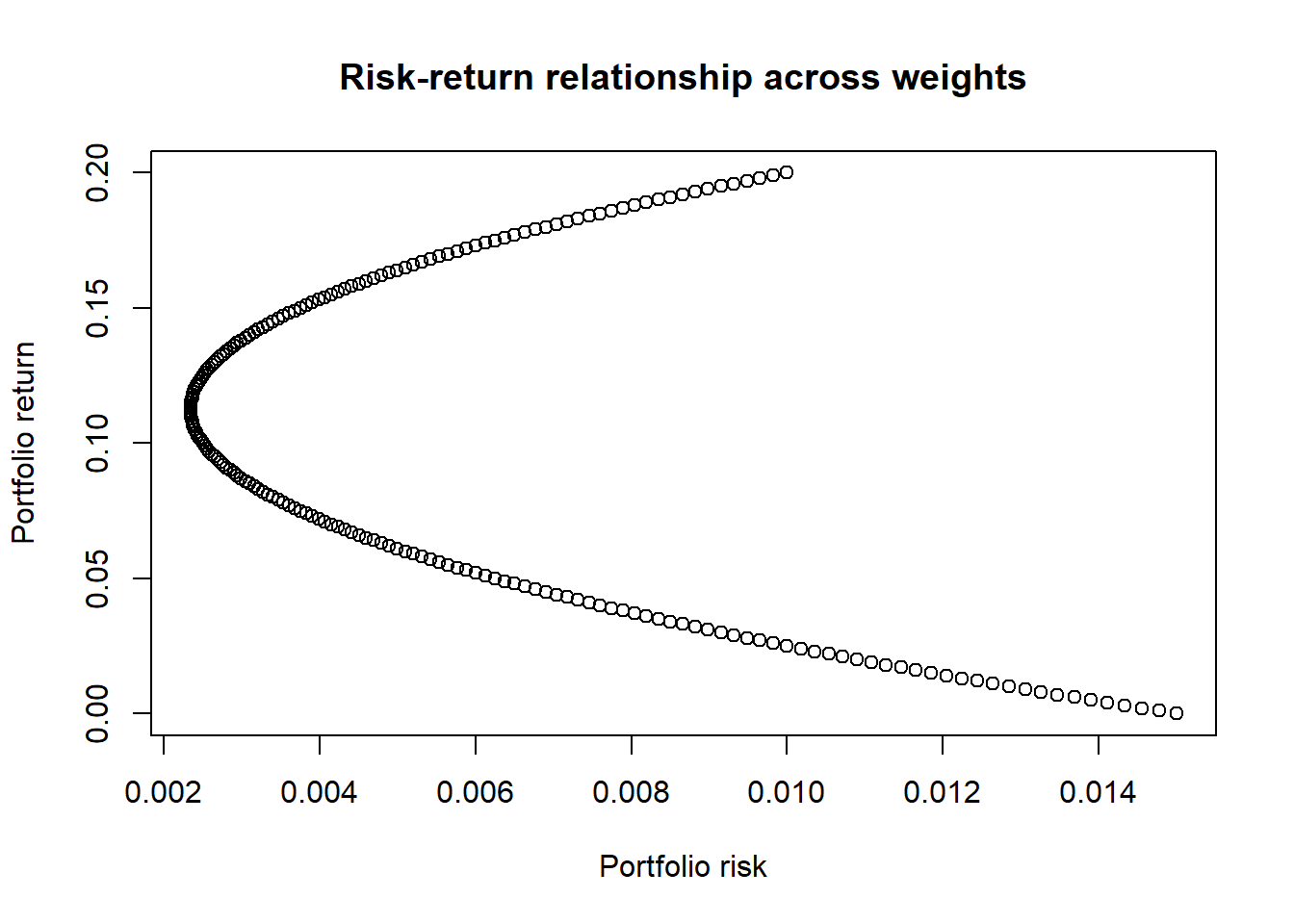
Efficient Portfolios
Take a look at the plot above. Notice that
- For every possible value of return, there is one corresponding value of risk.
- However, for every possible value of risk, there are two corresponding values of returns.
Naturally, for a given amount of risk that we would like to take on, we would want a higher return than a lower one. Therefore, any combination of risk-return that belongs to the top half of the plot would be portfolios that we would want, as compared to the lower half. In particular, each combination in the top half of the plot are considered as efficient portfolios. At this point, we might also want to know which is the portfolio or weight that has the lowest risks. This portfolio is also known as the minimum variance portfolio.
Terminology
Efficient portfolios lie on on the efficient frontier, the top half of our plot. By definition, the efficient frontier consists of portfolios such that for each of these portfolios and their respective returns, there exists no other portfolios that carries a lower portfolio risk for a given return (hence “efficient”5). The minimum variance portfolio is one special case of an efficient portfolio - no other portfolios carries a lower portfolio risk than itself, and is the leftmost point of our plot.
min_risk_w <- weights[which(risks == min(risks))]
min_risk_return <- mean(cal_pf_return(min_risk_w))

efficient_idx <- which(returns >= min_risk_return)
inefficient_idx <- which(returns < min_risk_return)

plot(risks[efficient_idx], returns[efficient_idx],
     xlab = "Portfolio risk",
     ylab = "Portfolio return",
     main = "The Efficient Frontier",
     ylim = c(0,0.2), xlim = c(0.002, 0.01))

lines(risks[inefficient_idx], returns[inefficient_idx], lty = "dotted")

abline(h = min_risk_return)
text(x = 0.003, y = min_risk_return-0.01, "min variance portfolio")
text(x = 0.006, y = 0.15, "efficient frontier")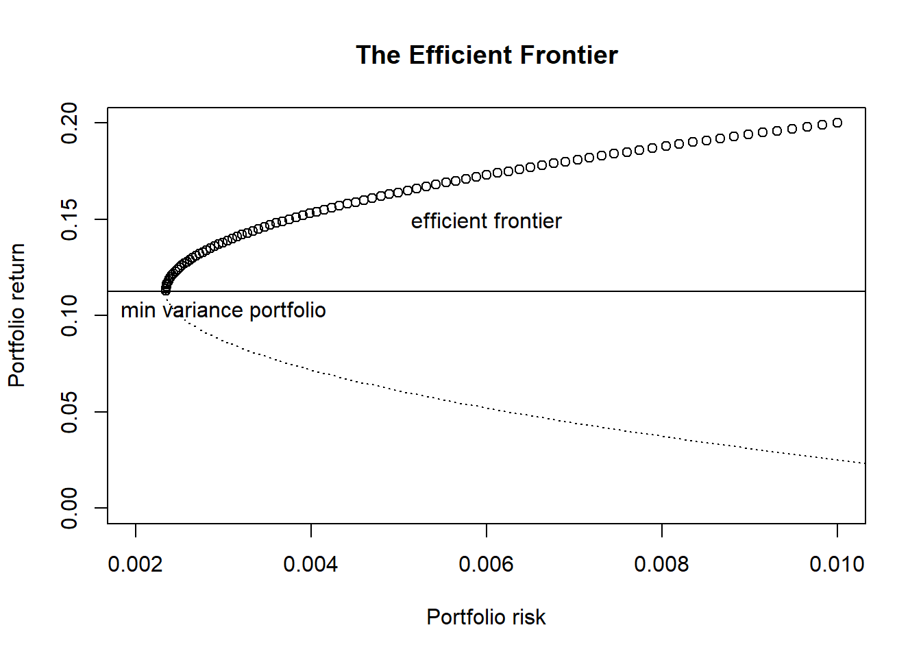
Minimum variance portfolio
In the example above, we arrived at the minimum variance portfolio by doing some simple calculations. A more robust method would be arrive at the minimum variance portfolio analytically by treating the problem as a optimization problem, minimizing \(Var(R_{pf})\). This can be done by simply solving some basic calculus.
\[ Var(R_{pf}) = w^2\sigma_1^2+ (1-w)^2\sigma_2^2 + 2w(1-w)\rho_{12}\sigma_1\sigma_2 \\ \frac{dVar(R_{pf})}{dw} = 2w\sigma_1^2 - 2(1-w)\sigma_2^2 + 2(1-2w)\rho_{12}\sigma_1\sigma_2 \\ \] Also, since
\[ \frac{d^2Var(R_{pf})}{dw^2} = 2\sigma_1^2 + 2\sigma_2^2 - 4\rho_{12}\sigma_1\sigma_2 \geqslant 2\sigma_1^2 + 2\sigma_2^2 - 4\sigma_1\sigma_2 = 2(\sigma_1 - \sigma_2)^2 \geqslant 0 \] where \(\rho_{12} < 1\). We would have \(\frac{d^2Var(R_{pf})}{dw^2} > 0\), i.e. solving \(\frac{dVar(R_{pf})}{dw} = 0\) minimizes \(Var(R_{pf})\), giving the minimium variance portfolio.
Solving,
\[ w \equiv w_{minvar} = \frac{\sigma_2^2 - \rho_{12}\sigma_1\sigma_2}{\sigma_1^2 + \sigma_2^2 - 2\rho_{12}\sigma_1\sigma_2} \] and
\[ 1 - w_{minvar} = \frac{\sigma_1^2 - \rho_{12}\sigma_1\sigma_2}{\sigma_1^2 + \sigma_2^2 - 2\rho_{12}\sigma_1\sigma_2} \]
Risk-free assets
Now let’s make this a little more interesting than just 2 assets. Since it’s always possible to not invest all our capital in these assets, and in fact leave a portion of capital in something that is risk-free, such as cash, we could include risk-free assets as part of our framework as well. In particular, we could have \(w_1 + w_2 < 1\), and \(1 - w_1 - w_2\) being the portion not invested, but instead diverted to risk-free assets. Doing this directly reduces portfolio variance, and of course reduces portfolio return.
Terminology
As pointed out above, risk-free assets are simply assets that are generally deemed as 100% safe6, such as cash in a deposit account7, Treasury Bills, or Singapore Savings Bonds. Typically, the three-month US Treasury Bills are used as proxies for risk-free assets, and their yield or return are considered accordingly. In context of Singapore, we could consider the yield of SSBs as risk-free returns.
Let \(R_{free}\) be the random variable representing the return of a risk-free asset. Then we have \(ER_{free} = \mu_{free}\), and \(Var(R_{free}) = 0\)8. Naturally, \(ER_{free}\) would be small and contributes a small return to portfolio. On the other hand, directly adjusting the \(1 - w_1 - w_2\) provides a convenient of controlling portfolio variance.
Also, note that since \(Var(R_{free}) = 0\), \(\forall i cov(R_{free}, R_i) = 0\), i.e. the risk-free is not correlated with any other “risky” assets9.
One “risky” asset and one risk-free asset
Now let’s consider combining a “risky” asset with a risk-free one. Let \(w\) be the weight invested in the risky asset, with its return being \(ER\) and variance being \(Var(R)\). The portfolio would look like this:
\[ ER_{pf} = wER + (1-w)R_{free} \implies \mu_{pf} = w\mu_R + (1-w)\mu_{free} \\ Var(R_{pf}) = w^2Var(R) \implies \sigma_{pf} = w\sigma_R \] In particular, observe that the portfolio variance is now a function of \(w\), i.e. solving \(Var(R_{pf}) = w^2Var(R)\) gives \(w = \frac{\sigma_{pf}}{\sigma_R}\), where \(\sigma_{pf}\) is the standard deviation of the portfolio and \(\sigma_R\) is the standard deviation of the risky asset.
This gives the following relationship between the portfolio return \(\mu_{pf}\) and variance \(\sigma_{pf}\):
\[ \mu_{pf} = \mu_{free} + \frac{\mu_R - \mu_{free}}{\sigma_R}\sigma_{pf} \] Again, let’s visualize this relationship with a numerical example.
# expected returns of both "risky" and risk-free asset, variance
mu_R    <- 0.2
mu_free <- 0.04
sigma_R <- 0.1

# calculate return and risks based on w
cal_pf_return <- function(w){
  return(w*mu_R + (1-w)*mu_free)
}
cal_pf_sd <- function(w){ # standard deviation, not variance
  return(w*sigma_R)
}

weights <- seq(0, 1, by = 0.01)

returns <- NULL
risks <- NULL

for(w in weights){
  returns <- c(returns, cal_pf_return(w))
  risks <- c(risks, cal_pf_sd(w))
}

plot(risks, returns,
     xlab = "Portfolio sd",
     ylab = "Portfolio return",
     main = "Risk-return relationship across weights")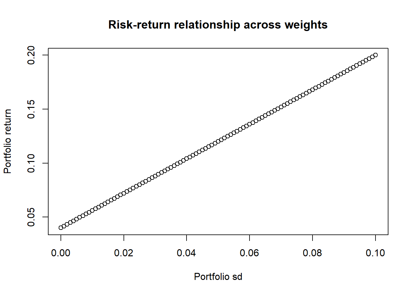
Two “risky” assets and one risk-free asset
Now, let’s go one step further, and look at having two “risky” assets with one risk-free asset. What does the math look like? Again, Let \(w_1\) be the weight invested in the first risky asset, \(w_2\) in the second risky asset and \(w_{free}\) in the risk-free asset, with respective returns being \(ER_1\), \(ER_2\) and \(ER_{free}\), and variances being \(Var(R_1)\) and \(Var(R_2)\).
Since there are now two risky assets, we also need to consider their correlation, \(\rho_{12}\). The portfolio would look like this:
\[ ER_{pf} = w_1ER_1 + w_2ER_2 + (1-w_1-w_2)R_{free} \implies \mu_{pf} = w_1\mu_{R_1} + w_2\mu_{R_2} + (1-w_1-w_2)\mu_{free} \\ Var(R_{pf}) = w_1^2Var(R_1) + w_2^2Var(R_2) + 2w_1w_2cov(R_1, R_2) = w_1^2\sigma_1^2 + w_2^2\sigma_2^2 + 2w_1w_2\rho_{12}\sigma_1\sigma_2 \\ w_{free} = 1-w_1-w_2 \] In particular, note that we can write \(ER_{pf}\) in the following manner as well:
\[ ER_{pf} = (1-w_{free})(\bar{w_1}R_1 + \bar{w_2}R_2) + w_{free}R_{free} \\ \bar{w_1} = \frac{w_1}{1-w_{free}}, \bar{w_2} = \frac{w_2}{1-w_{free}} \implies \bar{w_1} + \bar{w_2} = 1 \] In this sense, we can now view portfolio selection as a two-stage problem. First, we construct a portfolio based on risky assets only (e.g. chooosing \(\bar{w_1}\) and \(\bar{w_2}\) only). Then, we include the risk-free asset by choosing \(w_{free}\). From the perspective, we gain an interesting tool in controlling for the risk we take on in our portfolio, by the inclusion of the risk-free asset - since its inclusion always decreases the portfolio risk, regardless of the risky assets we take on.
Also note that once the first stage is completed, we are effectively dealing with one risky asset and one risk-free asset again, with the “single risky asset” being a combination of 2 risky assets, with \(\bar{w_1}\) and \(\bar{w_2}\).
Therefore, the scenario of using two risky assets and one risk-free asset simplifies that of using one risky asset and one risk-free asset! This results also generalises to \(N\) assets.
Conclusion
In this post, I have attempted to give a brief and hopefully gentle enough introduction to the Modern Portfolio Theory, using only statistics like mean, variance, and covariance. We looked at the math behind diversification, computed the Efficient Frontier, and generalised the problem from \(N=2\) assets to \(N>2\) assets.
If you are interested to go a bit further, you might want to find out more about the Tangency Portfolio and the Sharpe Ratio - both further extends our analysis and this post would have given you sufficient understanding for further exploration.
That’s all from me today, thank you for reading!
In my personal opinion, using standard deviation as a measure of risk is a little iffy, for several reasons. For example, risk could be better represented as a probability of huge losses, rather than the sd of expected returns - but let’s stick to this for now.↩
In particular, choosing \(w\) = \(\frac{1}{2}\) minimizes \(Var(R_{pf})\) at \(\frac{\sigma}{\sqrt{2}}\).↩
It’s commonly said that stocks and bonds are considered to be negatively correlated. Assuming this is true, consider the two subdomains \(\rho_{12} < 0\) and \(\rho_{12} > 0\). We have \(\forall\rho_{12} < 0, Var(R_{pf}) < \frac{1}{2}\sigma^2\) and \(\forall\rho_{12} > 0, Var(R_{pf}) > \frac{1}{2}\sigma^2\), i.e. portfolio risk reduces when you have two negatively correlated assets in the portfolio - an intuitive result and justification for proper diversification and strategic asset allocation. This of course begs the question on whether stocks and bonds are indeed negatively correlated, in good economic times and in bad, and correlated by how much. We can explore this topic deeper in the future. Also, the math here is similar to that of ensemble modelling in machine learning.↩
Of course the challenge in real life is to estimate them using historical data.↩
The same way an estimator \(\hat{\theta}\) is efficient if \(Var(\hat{\theta})\) is minimized.↩
Of course there is no such thing in real life.↩
We could in fact use a constant instead of a random variable.↩
Again, this is not always true in real life. For example, we have a coronavirus pandemic decimating the return of both “risky” and risk-free assets.↩