Introduction

Everyone knows what the average is. To find the average of the bunch of numbers, simply add them all up and then divide the total by the number of numbers there are. Calculating the average of a series of numbers has always been a straightforward way in which we summarize many numbers: “on average, I eat about 3 to 4 apples per week.” This calculating and reporting of the average summarizes a larger amount of information into a single summary - the mean itself.

Consider a series of say 9 numbers. Let’s call it v¹.

v <- c(2, 6, 9, 1, 10, 3, 3, 7, 8)
length(v)
## [1] 9

It makes sense to report the mean as a representative summary of a series of numbers.

mean(v)
## [1] 5.444444

Knowing the mean of something gives us some intuitive sense of the range of numbers that we are dealing with. For example, the mean definitely has to be within the series’ minimum (1) and maximum (10). With this, we also tend to associate the mean to be the “middle” of a series of numbers, whatever the “middle²” means.

In this post, I would like to illustrate a particular property of the mean that makes it a powerful single summary to describe a series of numbers, namely:

The mean minimizes the squared error.

At this point you may have some intuition on what’s about to follow, or it may not be immediately clear to you why this is important or what I am talking about. I will use a rather peculiar example to illustrate this property and its importance. Hopefully by the end of this example, it would be clearer.

As you read along, if you find this post a bit more abstract than my usual ones - my apologies!

A peculiar example

Consider the following diagram.

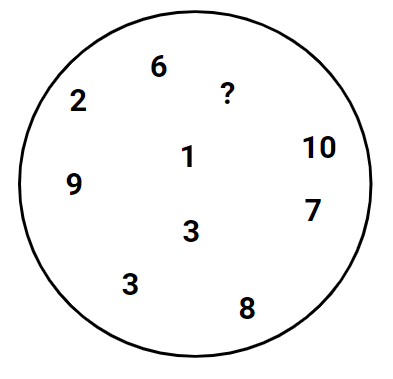
In this diagram, there are a bunch of numbers and a single question mark. Behind the question, is also a number. The known numbers are the same as in our friend v above.

Our task is as follows:

• Make a guess on what that mystery number could be. And,
• If we can’t get it right, then reduce, as much as possible, the error we incur on our guess.

Note that there is no special ordering or patterns in these numbers or their location in their circle. The only thing we know is that these numbers belong to a larger group of numbers, or that they all belong in a group with some other numbers unseen to us at the moment. (If it helps, you can think of them as being numbers relevant to something in real life, like the number of goldfishes that some fish owners have in their homes, out of all fish owners).

There are a few approaches to think about this strange and seemingly irrelevant problem:

1. Since 3 appeared twice, we should guess 3³.
2. Since 3 appeared twice, we should not guess 3.
3. Since we have no other information, any guess is as good as any other. For example, guessing 1,000,000 is the same as guessing 3 or 8 or any other number.
4. Given that we know these numbers belong together in some fashion, while the actual number could be anything - what is a good guess that reduces our error?

Remember, the only things we know now are as follows:

• These numbers belong to a larger group of other numbers.
• We want to minimize our error.

Let’s consider each of these approaches.

• Approach 1 - guess 3: frequentist, could work well. Keeping to the goldfish example, this assumes many fish owners keep 3 goldfishes, which, based on the information that we have, is an assumption. However, we can’t really use this as a rule for guessing since there’s no guarantee that duplicate numbers will always appear.
• Approach 2 - don’t guess 3: this assumes that we incidentally picked 3 twice, and the odds of 3 appearing again is low⁴. Then, with this, what should we guess? Kind of stuck.
• Approach 3 - it doesn’t matter, guess any number: this is useless as we can’t make any intelligent guess of any sorts.
• Approach 4 - what can reduce our error?: firstly, what does “belong to the same group” mean? The most intuitive way of extrapolating from that is that we can at least guess that the mystery number should be close to the other numbers of the circle - i.e. we have no reason to think that it’s smaller than the smallest number, or larger than the largest number, and have some intuition to guess that the mystery number is somewhere within the smallest and the largest number. A reasonable intuition.

So far so good? It seems like approaches 1 to 3 are not so helpful, and reducing error is our lead forward. At the least, approach 4 gives us some probable region of interest to guess, namely somewhere between the minimum 1 and maximium 10.

What then, minimizes the error? Well we must first define the error.

Minimizing our error

We are looking for a guess that reduces our error to as low as possible, given what we got. In an intuitive sense, we can define error to look something like

\[error = actual - guess\] Fair? We define the error to be distance or difference between the actual value, and our guess. The small the error, the closer our guess is to the actual value, whatever it may be.

What minimizes the squared error? - a simulation

To get a sense of this, let’s use some numerical simulation to get some intuition. Let’s bring our friend v back again.

v <- c(2, 6, 9, 1, 10, 3, 3, 7, 8)
length(v)
## [1] 9

Here, v contains all the numbers in the diagram above, in no particular order, other than question mark. A simple way to get some intuition here is simply to iteratively regard each of the 9 numbers in v as missing (i.e. a question mark), and use the remaining 8 numbers to make a guess, then validate our guess with the actual value. Confusing? Let me explain again, step-by-step:

v = (2, 6, 9, 1, 10, 3, 3, 7, 8)
1. Hide 2 and treat 2 as ?, use the rest of the numbers to guess, compare guess with actual value (2).
2. Hide 6 and treat 6 as ?, use the rest to guess, compare guess with actual (6).
3. Hide 9 and treat 9 as ?, use the rest to guess, compare guess with actual (9).
4. ...

By doing this, we get an interesting mechanic of iterating over different possibilities in order to learn something about our approach or objective of minimizing the squared error⁷.

Then for each step, let’s do many brute-force guesses, like this:

1. Hide 2 and treat 2 as ?, use the rest to guess, compare guess with actual value (2).
1.1. Guess 1, compare guess (1) with actual value (2), calculate squared error
1.2. Guess 2, compare guess (2) with actual value (2), calculate squared error
1.3. Guess 3, compare guess (3) with actual value (2), calculate squared error
...
1.10. Guess 10, compare guess (10) with actual value (2), calculate squared error

Step 2. Hide 6 and treat 6 as ?, use the rest to guess, compare guess with actual (6).
--->Step 2.1. ...

If it’s a little confusing, feel free to take a quick minute to think this through.

Let’s give it a shot and see what happens.

v <- c(2, 6, 9, 1, 10, 3, 3, 7, 8)
mean(v)
## [1] 5.444444
length(v)
## [1] 9

# leave-one-out, let's guess from 1 to 10?
# calculate error

simulation_set <- data.frame(leave_out = numeric(0),
                             guess = numeric(0),
                             error = numeric(0))

for(idx in seq_along(v)){
  leave_out <- v[idx]
  answer <- leave_out
  
  for(guess in 1:10){
    
    error <- guess - answer
    simulation_set <- rbind(simulation_set, data.frame(leave_out = leave_out, guess = guess, error = error))
  }
}

# calculate squared error
simulation_set$sq_error <- simulation_set$error**2
boxplot(simulation_set$sq_error ~ as.factor(simulation_set$guess), main = "Distribution of sq error for each guess (1 to 10)")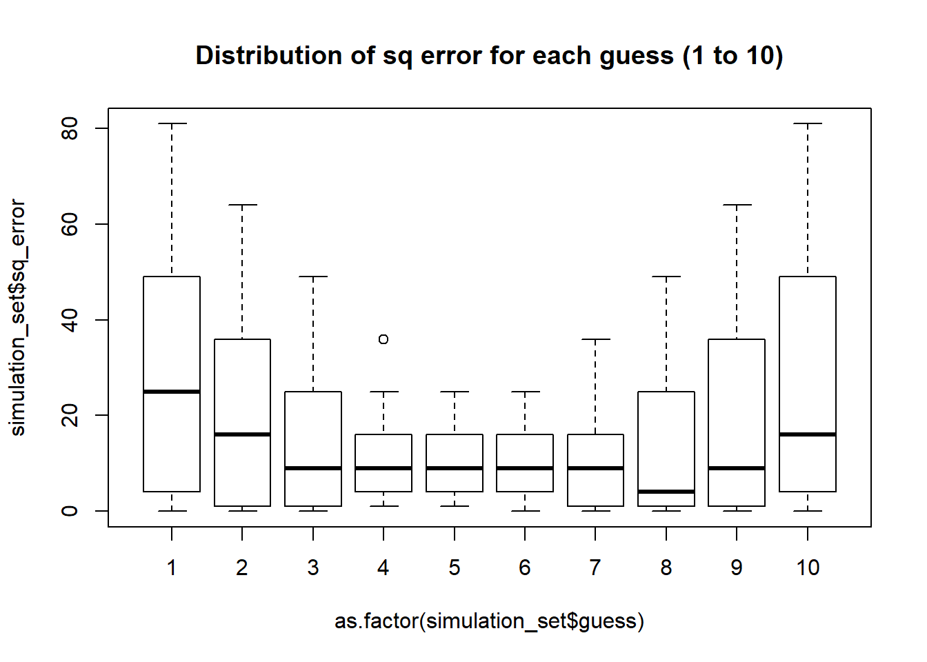

The plot above shows the distribution of squared error, as we use 1 to 10 as guesses⁸. Notice the U-shaped pattern here, where the error dips into the middle of the range, from 1 to 10.

Now we can get some sense of what may reduce or minimize our error in our initial problem - we would probably do well if we try to guess a number that is somewhere in the middle.

Alas, if we were to use the mean of our vector v, that is 5.4444444, here’s what it will look like:

v <- c(2, 6, 9, 1, 10, 3, 3, 7, 8)

simulation_set <- data.frame(leave_out = numeric(0),
                             guess = numeric(0),
                             error = numeric(0))

for(idx in seq_along(v)){
  leave_out <- v[idx]
  answer <- leave_out
  
  for(guess in c(1:10, mean(v))){ # including mean(v) here
    
    error <- guess - answer
    simulation_set <- rbind(simulation_set, data.frame(leave_out = leave_out, guess = guess, error = error))
  }
}

# calculate squared error
simulation_set$sq_error <- simulation_set$error**2
boxplot(simulation_set$sq_error ~ as.factor(simulation_set$guess),
        main = "Distribution of sq error for each guess (1 to 10), with the mean",
        names = c("1", "2", "3", "4", "5", "mean(v)", "6", "7", "8", "9", "10"),
        las = 2)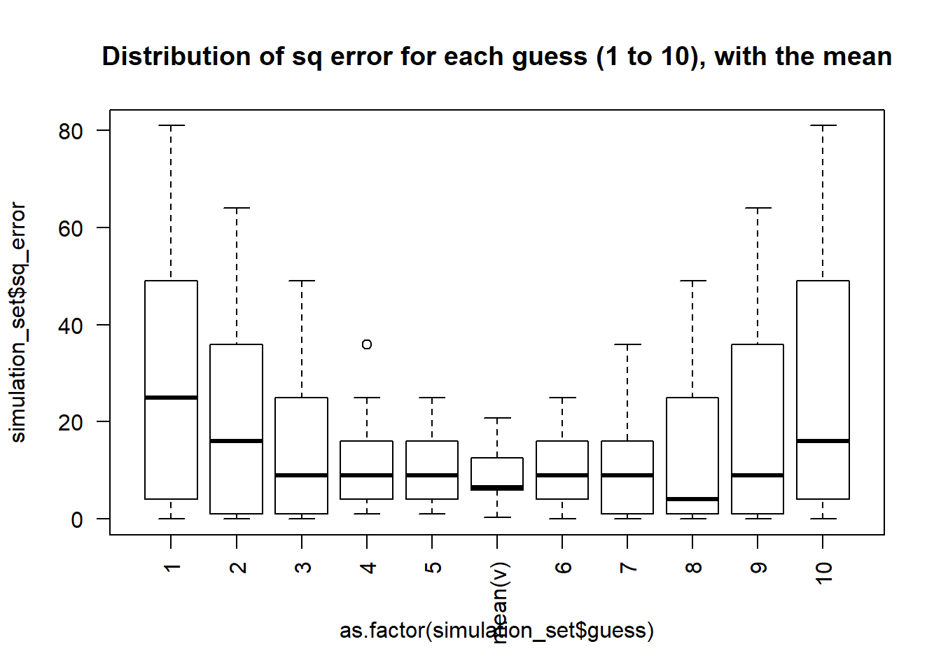

Here, we see that the mean does indeed minimize the squared error. What we have done so far is to replicate and show this property using simulation and brute force - the more elegant way would be to give prove the property mathematically, like in here.

Extensions and implications

Recall that we sort of have arbitarily chosen the squared error to be minimized, instead of the absolute error? Well if we have chosen the absolute error and conducted a similar simulation, we would have found that the median minimizes the absolute error. However, the squared error and the mean are much easier to work with, because the differentiability properties of the absolute and squared error - very very loosely speaking, the absolute error isn’t differentiable while the squared error is⁹. This has implications in linear regression modelling, which we can cover in a future post.

Finally, the purpose of using the average to represent a group of numbers is so that we can remain basically as close to the numbers within that group as possible, while taking into account all at once the numbers in that group.

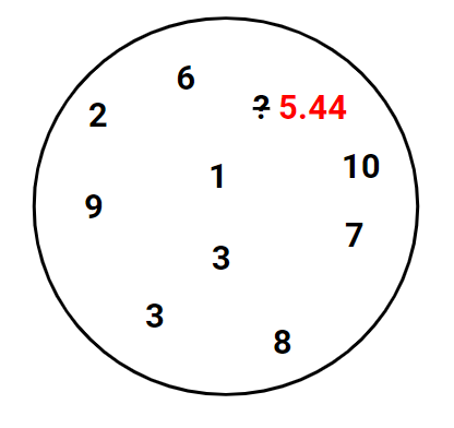
This also means that in our initial problem of guessing what’s the number behind the question mark, the best guess that can be used to minimize our error would be use all the known numbers in the circle, calculate the mean, and use that as our guess.